Python API¶

This section includes information for using the pure Python API of bob.math.

Summary¶

`bob.math.LPInteriorPoint`	Base class to solve a linear program using interior point methods.
`bob.math.LPInteriorPointShortstep`	A Linear Program solver based on a short step interior point method.
`bob.math.LPInteriorPointLongstep`	A Linear Program solver based on a long step interior point method.
`bob.math.chi_square`	chi_square(h1, h2) -> dist
`bob.math.svd`
`bob.math.gsvd`
`bob.math.histogram_intersection`	histogram_intersection(h1, h2) -> sim
`bob.math.kullback_leibler`	kullback_leibler(h1, h2) -> dist
`bob.math.linsolve`	linsolve(A, b) -> x
`bob.math.linsolve_cg_sympos`	linsolve_cg_sympos(A, b) -> x
`bob.math.linsolve_sympos`	linsolve_sympos(A, b) -> x
`bob.math.norminv`((p, mu, sigma) -> inv)	Computes the inverse normal cumulative distribution
`bob.math.pavx`	pavx(input, output) -> None
`bob.math.pavxWidth`((input, output) -> width)	Applies the Pool-Adjacent-Violators Algorithm and returns the width.
`bob.math.pavxWidthHeight`((input, ...)	Applies the Pool-Adjacent-Violators Algorithm and returns the width and the height.
`bob.math.scatter`	scatter(a) -> s, m
`bob.math.scatters`	scatters(data) -> sw, sb, m

Details¶

bob.math.get_config()[source]¶: Returns a string containing the configuration information.

class bob.math.LPInteriorPoint¶

Bases: object

Base class to solve a linear program using interior point methods.

For more details about the algorithms,please refer to the following book: ‘Primal-Dual Interior-Point Methods’, Stephen J. Wright, ISBN: 978-0898713824, Chapter 5, ‘Path-Following Algorithms’.

Warning

You cannot instantiate an object of this type directly, you must use it through one of the inherited types.

The primal linear program (LP) is defined as follows:

$\min c^T*x \text{, s.t. } A*x=b, x>=0$

The dual formulation is:

$\min b^T*\lambda \text{, s.t. } A^T*\lambda+\mu=c$

Class Members:

epsilon¶: float <– The precision to determine whether an equality constraint is fulfilled or not

initialize_dual_lambda_mu(A, c) → None¶: Initializes the dual variables lambda and mu by minimizing the logarithmic barrier function.

is_feasible(A, b, c, x, lambda, mu) → test¶

Checks if a primal-dual point (x, lambda, mu) belongs to the set of feasible points (i.e. fulfills the constraints).

Returns:

test : bool

True if (x, labmda, mu) belongs to the set of feasible points, otherwise False

is_in_v(x, mu, theta) → test¶

Checks if a primal-dual point (x, lambda, mu) belongs to the V2 neighborhood of the central path.

Returns:

test : bool

True if (x, labmda, mu) belongs to the V2 neighborhood of the central path, otherwise False

is_in_v_s(A, b, c, x, lambda, mu) → test¶

Checks if a primal-dual point (x,lambda,mu) belongs to the V neighborhood of the central path and the set of feasible points.

Returns:

test : bool

True if (x, labmda, mu) belongs to the V neighborhood of the central path and the set of feasible points, otherwise False

lambda_¶: float <– The value of the $\lambda$ dual variable (read-only)

m¶: int <– The first dimension of the problem/A matrix

mu¶: float <– The value of the $\mu$ dual variable (read-only)

n¶: int <– The second dimension of the problem/A matrix

reset(M, N) → None¶

Resets the size of the problem (M and N correspond to the dimensions of the A matrix)

Parameters:

M : int

The new first dimension of the problem/A matrix

N : int

The new second dimension of the problem/A matrix

solve(A, b, c, x0, lambda, mu) → x¶

Solves an LP problem

Parameters:

lambda : ?, optional

mu : ?, optional

class bob.math.LPInteriorPointLongstep¶

Bases: bob.math.LPInteriorPoint

A Linear Program solver based on a long step interior point method.

See LPInteriorPoint for more details on the base class.

Constructor Documentation:

bob.math.LPInteriorPointLongstep (M, N, gamma, sigma, epsilon)

bob.math.LPInteriorPointLongstep (solver)

Objects of this class can be initialized in two different ways: a detailed constructor with the parameters described below or a copy constructor, that deep-copies the input object and creates a new object (not a new reference to the same object)

Parameters:

M : int

first dimension of the A matrix

N : int

second dimension of the A matrix

gamma : float

the value gamma used to define a V-inf neighborhood

sigma : float

the value sigma used to define a V-inf neighborhood

epsilon : float

the precision to determine whether an equality constraint is fulfilled or not

solver : LPInteriorPointLongstep

the solver to make a deep copy of

Class Members:

epsilon¶: float <– The precision to determine whether an equality constraint is fulfilled or not

gamma¶: float <– The value gamma used to define a V-Inf neighborhood

initialize_dual_lambda_mu(A, c) → None¶: Initializes the dual variables lambda and mu by minimizing the logarithmic barrier function.

is_feasible(A, b, c, x, lambda, mu) → test¶

Checks if a primal-dual point (x, lambda, mu) belongs to the set of feasible points (i.e. fulfills the constraints).

Returns:

test : bool

True if (x, labmda, mu) belongs to the set of feasible points, otherwise False

is_in_v(x, mu, gamma) → test¶

Checks if a primal-dual point (x, lambda, mu) belongs to the V-Inf neighborhood of the central path.

Returns:

test : bool

True if (x, lambda, mu) belong to the V-Inf neighborhood of the central path, otherwise False

is_in_v_s(A, b, c, x, lambda, mu) → test¶

Checks if a primal-dual point (x,lambda,mu) belongs to the V neighborhood of the central path and the set of feasible points.

Returns:

test : bool

True if (x, labmda, mu) belongs to the V neighborhood of the central path and the set of feasible points, otherwise False

lambda_¶: float <– The value of the $\lambda$ dual variable (read-only)

m¶: int <– The first dimension of the problem/A matrix

mu¶: float <– The value of the $\mu$ dual variable (read-only)

n¶: int <– The second dimension of the problem/A matrix

reset(M, N) → None¶

Resets the size of the problem (M and N correspond to the dimensions of the A matrix)

Parameters:

M : int

The new first dimension of the problem/A matrix

N : int

The new second dimension of the problem/A matrix

sigma¶: float <– The value sigma used to define a V-Inf neighborhood

solve(A, b, c, x0, lambda, mu) → x¶

Solves an LP problem

Parameters:

lambda : ?, optional

mu : ?, optional

class bob.math.LPInteriorPointPredictorCorrector¶

Bases: bob.math.LPInteriorPoint

A Linear Program solver based on a predictor-corrector interior point method.

See LPInteriorPoint for more details on the base class.

Constructor Documentation:

bob.math.LPInteriorPointPredictorCorrector (M, N, theta_pred, theta_corr, epsilon)

bob.math.LPInteriorPointPredictorCorrector (solver)

Objects of this class can be initialized in two different ways: a detailed constructor with the parameters described below or a copy constructor, that deep-copies the input object and creates a new object (not a new reference to the same object).

Parameters:

M : int

first dimension of the A matrix

N : int

second dimension of the A matrix

theta_pred : float

the value theta_pred used to define a V2 neighborhood

theta_corr : float

the value theta_corr used to define a V2 neighborhood

epsilon : float

the precision to determine whether an equality constraint is fulfilled or not

solver : LPInteriorPointPredictorCorrector

the solver to make a deep copy of

Class Members:

epsilon¶: float <– The precision to determine whether an equality constraint is fulfilled or not

initialize_dual_lambda_mu(A, c) → None¶: Initializes the dual variables lambda and mu by minimizing the logarithmic barrier function.

is_feasible(A, b, c, x, lambda, mu) → test¶

Checks if a primal-dual point (x, lambda, mu) belongs to the set of feasible points (i.e. fulfills the constraints).

Returns:

test : bool

True if (x, labmda, mu) belongs to the set of feasible points, otherwise False

is_in_v(x, mu, theta) → test¶

Checks if a primal-dual point (x, lambda, mu) belongs to the V2 neighborhood of the central path.

Returns:

test : bool

True if (x, labmda, mu) belongs to the V2 neighborhood of the central path, otherwise False

is_in_v_s(A, b, c, x, lambda, mu) → test¶

Checks if a primal-dual point (x,lambda,mu) belongs to the V neighborhood of the central path and the set of feasible points.

Returns:

test : bool

True if (x, labmda, mu) belongs to the V neighborhood of the central path and the set of feasible points, otherwise False

lambda_¶: float <– The value of the $\lambda$ dual variable (read-only)

m¶: int <– The first dimension of the problem/A matrix

mu¶: float <– The value of the $\mu$ dual variable (read-only)

n¶: int <– The second dimension of the problem/A matrix

reset(M, N) → None¶

Resets the size of the problem (M and N correspond to the dimensions of the A matrix)

Parameters:

M : int

The new first dimension of the problem/A matrix

N : int

The new second dimension of the problem/A matrix

solve(A, b, c, x0, lambda, mu) → x¶

Solves an LP problem

Parameters:

lambda : ?, optional

mu : ?, optional

theta_corr¶: float <– The value theta_corr used to define a V2 neighborhood

theta_pred¶: float <– The value theta_pred used to define a V2 neighborhood

class bob.math.LPInteriorPointShortstep¶

Bases: bob.math.LPInteriorPoint

A Linear Program solver based on a short step interior point method. See LPInteriorPoint for more details on the base class.

Constructor Documentation:

bob.math.LPInteriorPointShortstep (M, N, theta, epsilon)

bob.math.LPInteriorPointShortstep (solver)

Objects of this class can be initialized in two different ways: a detailed constructor with the parameters described below or a copy constructor that deep-copies the input object and creates a new object (not a new reference to the same object).

Parameters:

M : int

first dimension of the A matrix

N : int

second dimension of the A matrix

theta : float

The value defining the size of the V2 neighborhood

epsilon : float

The precision to determine whether an equality constraint is fulfilled or not.

solver : LPInteriorPointShortstep

The solver to make a deep copy of

Class Members:

Highlighted Methods:

solve() Solves an LP problem

Highlighted Attributes:

mu The value of the $\mu$ dual variable (read-only)

lambda_ The value of the $\lambda$ dual variable (read-only)

epsilon¶: float <– The precision to determine whether an equality constraint is fulfilled or not

initialize_dual_lambda_mu(A, c) → None¶: Initializes the dual variables lambda and mu by minimizing the logarithmic barrier function.

is_feasible(A, b, c, x, lambda, mu) → test¶

Checks if a primal-dual point (x, lambda, mu) belongs to the set of feasible points (i.e. fulfills the constraints).

Returns:

test : bool

True if (x, labmda, mu) belongs to the set of feasible points, otherwise False

is_in_v(x, mu, theta) → test¶

Checks if a primal-dual point (x, lambda, mu) belongs to the V2 neighborhood of the central path.

Returns:

test : bool

True if (x, labmda, mu) belongs to the V2 neighborhood of the central path, otherwise False

is_in_v_s(A, b, c, x, lambda, mu) → test¶

Checks if a primal-dual point (x,lambda,mu) belongs to the V neighborhood of the central path and the set of feasible points.

Returns:

test : bool

True if (x, labmda, mu) belongs to the V neighborhood of the central path and the set of feasible points, otherwise False

lambda_¶: float <– The value of the $\lambda$ dual variable (read-only)

m¶: int <– The first dimension of the problem/A matrix

mu¶: float <– The value of the $\mu$ dual variable (read-only)

n¶: int <– The second dimension of the problem/A matrix

reset(M, N) → None¶

Resets the size of the problem (M and N correspond to the dimensions of the A matrix)

Parameters:

M : int

The new first dimension of the problem/A matrix

N : int

The new second dimension of the problem/A matrix

solve(A, b, c, x0, lambda, mu) → x¶

Solves an LP problem

Parameters:

lambda : ?, optional

mu : ?, optional

theta¶: float <– The value theta used to define a V2 neighborhood

bob.math.chi_square()¶

chi_square(h1, h2) -> dist
chi_square(index_1, value_1, index_2, value_2) -> dist

Computes the chi square distance between the given histograms, which might be of singular dimension only.

The chi square distance is computed as follows:

$dist(h_1,h_2) = \sum_i \frac{(h_{1i} - h_{2i})^2}{h_{1i} + h_{2i}}$

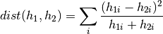
Chi square defines a distance metric, so lower values are better. You can use this method in two different formats. The first interface accepts non-sparse histograms. The second interface accepts sparse histograms represented by indexes and values.

Note

Histograms are given as two matrices, one with the indexes and one with the data. All data points that for which no index exists are considered to be zero.

Note

In general, histogram intersection with sparse histograms needs more time to be computed.

Parameters:

h1, h2 : array_like (1D)

Histograms to compute the chi square distance for

index_1, index_2 : array_like (int, 1D)

Indices of the sparse histograms value_1 and value_2

value_1, value_2 : array_like (1D)

Sparse histograms to compute the chi square distance for

Returns:

dist : float

The chi square distance value for the given histograms.

bob.math.histogram_intersection()¶

histogram_intersection(h1, h2) -> sim
histogram_intersection(index_1, value_1, index_2, value_2) -> sim

Computes the histogram intersection between the given histograms, which might be of singular dimension only.

The histogram intersection is computed as follows:

$sim(h_1,h_2) = \sum_i \min \{h_{1i}, h_{2i}\}$

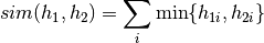
The histogram intersection defines a similarity measure, so higher values are better. You can use this method in two different formats. The first interface accepts non-sparse histograms. The second interface accepts sparse histograms represented by indexes and values.

Note

Histograms are given as two matrices, one with the indexes and one with the data. All data points that for which no index exists are considered to be zero.

Note

In general, histogram intersection with sparse histograms needs more time to be computed.

Parameters:

h1, h2 : array_like (1D)

Histograms to compute the histogram intersection for

index_1, index_2 : array_like (int, 1D)

Indices of the sparse histograms value_1 and value_2

value_1, value_2 : array_like (1D)

Sparse histograms to compute the histogram intersection for

Returns:

sim : float

The histogram intersection value for the given histograms.

bob.math.kullback_leibler()¶

kullback_leibler(h1, h2) -> dist
kullback_leibler(index_1, value_1, index_2, value_2) -> dist

Computes the Kullback-Leibler histogram divergence between the given histograms, which might be of singular dimension only.

The chi square distance is inspired by link and computed as follows:

$dist(h_1,h_2) = \sum_i (h_{1i} - h_{2i}) * \log (h_{1i} / h_{2i})$

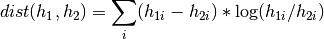
The Kullback-Leibler divergence defines a distance metric, so lower values are better. You can use this method in two different formats. The first interface accepts non-sparse histograms. The second interface accepts sparse histograms represented by indexes and values.

Note

Histograms are given as two matrices, one with the indexes and one with the data. All data points that for which no index exists are considered to be zero.

Note

In general, histogram intersection with sparse histograms needs more time to be computed.

Parameters:

h1, h2 : array_like (1D)

Histograms to compute the Kullback-Leibler divergence for

index_1, index_2 : array_like (int, 1D)

Indices of the sparse histograms value_1 and value_2

value_1, value_2 : array_like (1D)

Sparse histograms to compute the Kullback-Leibler divergence for

Returns:

dist : float

The Kullback-Leibler divergence value for the given histograms.

bob.math.linsolve()¶

linsolve(A, b) -> x
linsolve(A, b, x) -> None

Solves the linear system $Ax=b$ and returns the result in $x$ .

This method uses LAPACK’s dgesv generic solver. You can use this method in two different formats. The first interface accepts the matrices $A$ and $b$ returning $x$ . The second one accepts a pre-allocated $x$ vector and sets it with the linear system solution.

Parameters:

A : array_like (2D)

The matrix $A$ of the linear system

b : array_like (1D)

The vector $b$ of the linear system

x : array_like (1D)

The result vector $x$ , as parameter

Returns:

x : array_like (1D)

The result vector $x$ , as return value

bob.math.linsolve_()¶

linsolve_(A, b) -> x
linsolve_(A, b, x) -> None

Solves the linear system $Ax=b$ and returns the result in $x$ .

Warning

This variant does not perform any checks on the input matrices and is faster then linsolve(). Use it when you are sure your input matrices sizes match.

This method uses LAPACK’s dgesv generic solver. You can use this method in two different formats. The first interface accepts the matrices $A$ and $b$ returning $x$ . The second one accepts a pre-allocated $x$ vector and sets it with the linear system solution.

Parameters:

A : array_like (2D)

The matrix $A$ of the linear system

b : array_like (1D)

The vector $b$ of the linear system

x : array_like (1D)

The result vector $x$ , as parameter

Returns:

x : array_like (1D)

The result vector $x$ , as return value

bob.math.linsolve_cg_sympos()¶

linsolve_cg_sympos(A, b) -> x
linsolve_cg_sympos(A, b, x) -> None

Solves the linear system $Ax=b$ using conjugate gradients and returns the result in $x$ for symmetric $A$ matrix.

This method uses the conjugate gradient solver, assuming $A$ is a symmetric positive definite matrix. You can use this method in two different formats. The first interface accepts the matrices $A$ and $b$ returning $x$ . The second one accepts a pre-allocated $x$ vector and sets it with the linear system solution.

Parameters:

A : array_like (2D)

The matrix $A$ of the linear system

b : array_like (1D)

The vector $b$ of the linear system

x : array_like (1D)

The result vector $x$ , as parameter

Returns:

x : array_like (1D)

The result vector $x$ , as return value

bob.math.linsolve_cg_sympos_()¶

linsolve_cg_sympos_(A, b) -> x
linsolve_cg_sympos_(A, b, x) -> None

Solves the linear system $Ax=b$ using conjugate gradients and returns the result in $x$ for symmetric $A$ matrix.

Warning

This variant does not perform any checks on the input matrices and is faster then linsolve_cg_sympos(). Use it when you are sure your input matrices sizes match.

This method uses the conjugate gradient solver, assuming $A$ is a symmetric positive definite matrix. You can use this method in two different formats. The first interface accepts the matrices $A$ and $b$ returning $x$ . The second one accepts a pre-allocated $x$ vector and sets it with the linear system solution.

Parameters:

A : array_like (2D)

The matrix $A$ of the linear system

b : array_like (1D)

The vector $b$ of the linear system

x : array_like (1D)

The result vector $x$ , as parameter

Returns:

x : array_like (1D)

The result vector $x$ , as return value

bob.math.linsolve_sympos()¶

linsolve_sympos(A, b) -> x
linsolve_sympos(A, b, x) -> None

Solves the linear system $Ax=b$ and returns the result in $x$ for symmetric $A$ matrix.

This method uses LAPACK’s dposv solver, assuming $A$ is a symmetric positive definite matrix. You can use this method in two different formats. The first interface accepts the matrices $A$ and $b$ returning $x$ . The second one accepts a pre-allocated $x$ vector and sets it with the linear system solution.

Parameters:

A : array_like (2D)

The matrix $A$ of the linear system

b : array_like (1D)

The vector $b$ of the linear system

x : array_like (1D)

The result vector $x$ , as parameter

Returns:

x : array_like (1D)

The result vector $x$ , as return value

bob.math.linsolve_sympos_()¶

linsolve_sympos_(A, b) -> x
linsolve_sympos_(A, b, x) -> None

Solves the linear system $Ax=b$ and returns the result in $x$ for symmetric $A$ matrix.

Warning

This variant does not perform any checks on the input matrices and is faster then linsolve_sympos(). Use it when you are sure your input matrices sizes match.

This method uses LAPACK’s dposv solver, assuming $A$ is a symmetric positive definite matrix. You can use this method in two different formats. The first interface accepts the matrices $A$ and $b$ returning $x$ . The second one accepts a pre-allocated $x$ vector and sets it with the linear system solution.

Parameters:

A : array_like (2D)

The matrix $A$ of the linear system

b : array_like (1D)

The vector $b$ of the linear system

x : array_like (1D)

The result vector $x$ , as parameter

Returns:

x : array_like (1D)

The result vector $x$ , as return value

bob.math.norminv(p, mu, sigma) → inv¶

Computes the inverse normal cumulative distribution

Computes the inverse normal cumulative distribution for a probability $p$ , given a distribution with mean $\mu$ and standard deviation $\sigma$ . Reference: http://home.online.no/~pjacklam/notes/invnorm/

Parameters:

p : float

The value to get the inverse distribution of, must lie in the range $[0,1]$

mu : float

The mean $\mu$ of the normal distribution

sigma : float

The standard deviation $\sigma$ of the normal distribution

Returns:

inv : float

The inverse of the normal distribution

bob.math.normsinv(p) → inv¶

Computes the inverse normal cumulative distribution

Computes the inverse normal cumulative distribution for a probability $p$ , given a distribution with mean $\mu=0$ and standard deviation $\sigma=1$ . It is equivalent as calling norminv(p, 0, 1) (see norminv()). Reference: http://home.online.no/~pjacklam/notes/invnorm/

Parameters:

p : float

The value to get the inverse distribution of, must lie in the range $[0,1]$

Returns:

inv : float

The inverse of the normal distribution

bob.math.pavx()¶

pavx(input, output) -> None
pavx(input) -> output

Applies the Pool-Adjacent-Violators Algorithm

Applies the Pool-Adjacent-Violators Algorithm to input. This is a simplified C++ port of the isotonic regression code made available at the University of Bern website.

You can use this method in two different formats. The first interface accepts the input and output. The second one accepts the input array input and allocates a new output array, which is returned.

Parameters:

input : array_like (float, 1D)

The input matrix for the PAV algorithm.

output : array_like (float, 1D)

The output matrix, must be of the same size as input

Returns:

output : array_like (float, 1D)

The output matrix; will be created in the same size as input

bob.math.pavxWidth(input, output) → width¶

Applies the Pool-Adjacent-Violators Algorithm and returns the width.

Applies the Pool-Adjacent-Violators Algorithm to input. This is a simplified C++ port of the isotonic regression code made available at the University of Bern website.

Parameters:

input : array_like (float, 1D)

The input matrix for the PAV algorithm.

output : array_like (float, 1D)

The output matrix, must be of the same size as input

Returns:

width : array_like (uint64, 1D)

The width matrix will be created in the same size as input

bob.math.pavxWidthHeight(input, output) → width, height¶

Applies the Pool-Adjacent-Violators Algorithm and returns the width and the height.

Applies the Pool-Adjacent-Violators Algorithm to input. This is a simplified C++ port of the isotonic regression code made available at the University of Bern website.

Parameters:

input : array_like (float, 1D)

The input matrix for the PAV algorithm.

output : array_like (float, 1D)

The output matrix, must be of the same size as input

Returns:

width : array_like (uint64, 1D)

The width matrix will be created in the same size as input

height : array_like (float, 1D)

The height matrix will be created in the same size as input

bob.math.pavx_()¶

pavx_(input, output) -> None
pavx_(input) -> output

Applies the Pool-Adjacent-Violators Algorithm

Warning

This variant does not perform any checks on the input matrices and is faster then pavx(). Use it when you are sure your input matrices sizes match.

Applies the Pool-Adjacent-Violators Algorithm to input. This is a simplified C++ port of the isotonic regression code made available at the University of Bern website.

You can use this method in two different formats. The first interface accepts the input and output. The second one accepts the input array input and allocates a new output array, which is returned.

Parameters:

input : array_like (float, 1D)

The input matrix for the PAV algorithm.

output : array_like (float, 1D)

The output matrix, must be of the same size as input

Returns:

output : array_like (float, 1D)

The output matrix; will be created in the same size as input

bob.math.scatter()¶

scatter(a) -> s, m
scatter(a, s) -> m
scatter(a, m) -> s
scatter(a, s, m) -> None

Computes scatter matrix of a 2D array.

Computes the scatter matrix of a 2D array considering data is organized row-wise (each sample is a row, each feature is a column). The resulting array s is squared with extents equal to the number of columns in a. The resulting array m is a 1D array with the row means of a. This function supports many calling modes, but you should provide, at least, the input data matrix a. All non-provided arguments will be allocated internally and returned.

Parameters:

a : array_like (float, 2D)

The sample matrix, considering data is organized row-wise (each sample is a row, each feature is a column)

s : array_like (float, 2D)

The scatter matrix, squared with extents equal to the number of columns in a

m : array_like (float,1D)

The mean matrix, with with the row means of a

Returns:

s : array_like (float, 2D)

The scatter matrix, squared with extents equal to the number of columns in a

m : array_like (float, 1D)

The mean matrix, with with the row means of a

bob.math.scatter_(a, s, m) → None¶

Computes scatter matrix of a 2D array.

Warning

This variant does not perform any checks on the input matrices and is faster then scatter().Use it when you are sure your input matrices sizes match.

Computes the scatter matrix of a 2D array considering data is organized row-wise (each sample is a row, each feature is a column). The resulting array s is squared with extents equal to the number of columns in a. The resulting array m is a 1D array with the row means of a. This function supports many calling modes, but you should provide, at least, the input data matrix a. All non-provided arguments will be allocated internally and returned.

Parameters:

a : array_like (float, 2D)

The sample matrix, considering data is organized row-wise (each sample is a row, each feature is a column)

s : array_like (float, 2D)

The scatter matrix, squared with extents equal to the number of columns in a

m : array_like (float,1D)

The mean matrix, with with the row means of a

bob.math.scatters()¶

scatters(data) -> sw, sb, m
scatters(data, sw, sb) -> m
scatters(data, sw, sb, m) -> None

Computes $S_w$ and $S_b$ scatter matrices of a set of 2D arrays.

Computes the within-class $S_w$ and between-class $S_b$ scatter matrices of a set of 2D arrays considering data is organized row-wise (each sample is a row, each feature is a column), and each matrix contains data of one class. Computes the scatter matrix of a 2D array considering data is organized row-wise (each sample is a row, each feature is a column). The implemented strategy is:

Evaluate the overall mean (m), class means ( $m_k$ ) and the

total class counts ( $N$ ).
Evaluate sw and sb using normal loops.

Note that in this implementation, sw and sb will be normalized by N-1 (number of samples) and K (number of classes). This procedure makes the eigen values scaled by (N-1)/K, effectively increasing their values. The main motivation for this normalization are numerical precision concerns with the increasing number of samples causing a rather large $S_w$ matrix. A normalization strategy mitigates this problem. The eigen vectors will see no effect on this normalization as they are normalized in the euclidean sense ( $||a|| = 1$ ) so that does not change those.

This function supports many calling modes, but you should provide, at least, the input data. All non-provided arguments will be allocated internally and returned.

Parameters:

data : [array_like (float, 2D)]

The list of sample matrices. In each sample matrix the data is organized row-wise (each sample is a row, each feature is a column). Each matrix stores the data of a particular class. Every matrix in ``data`` must have exactly the same number of columns.

sw : array_like (float, 2D)

The within-class scatter matrix $S_w$ , squared with extents equal to the number of columns in data

sb : array_like (float, 2D)

The between-class scatter matrix $S_b$ , squared with extents equal to the number of columns in data

m : array_like (float,1D)

The mean matrix, representing the ensemble mean with no prior (i.e., biased towards classes with more samples)

Returns:

sw : array_like (float, 2D)

The within-class scatter matrix $S_w$

sb : array_like (float, 2D)

The between-class scatter matrix $S_b$

m : array_like (float, 1D)

The mean matrix, representing the ensemble mean with no prior (i.e., biased towards classes with more samples)

bob.math.scatters_()¶

scatters_(data, sw, sb, m) -> None
scatters_(data, sw, sb) -> None

Computes $S_w$ and $S_b$ scatter matrices of a set of 2D arrays.

Warning

This variant does not perform any checks on the input matrices and is faster then scatters(). Use it when you are sure your input matrices sizes match.

For a detailed description of the function, please see scatters().

Parameters:

data : [array_like (float, 2D)]

The list of sample matrices. In each sample matrix the data is organized row-wise (each sample is a row, each feature is a column). Each matrix stores the data of a particular class. Every matrix in ``data`` must have exactly the same number of columns.

sw : array_like (float, 2D)

The within-class scatter matrix $S_w$ , squared with extents equal to the number of columns in data

sb : array_like (float, 2D)

The between-class scatter matrix $S_b$ , squared with extents equal to the number of columns in data

m : array_like (float,1D)

The mean matrix, representing the ensemble mean with no prior (i.e., biased towards classes with more samples)

Python API¶

Summary¶

Details¶

Table Of Contents

Previous topic

Next topic

This Page