User Guide
Methods in the bob.measure module can help you to quickly and easily
evaluate error for multi-class or binary classification problems. If you are
not yet familiarized with aspects of performance evaluation, we recommend the
following papers and book chapters for an overview of some of the implemented
methods.
- Bengio, S., Keller, M., Mariéthoz, J. (2004). The Expected Performance Curve. International Conference on Machine Learning ICML Workshop on ROC Analysis in Machine Learning, 136(1), 1963–1966.
- Martin, A., Doddington, G., Kamm, T., Ordowski, M., & Przybocki, M. (1997). The DET curve in assessment of detection task performance. Fifth European Conference on Speech Communication and Technology (pp. 1895-1898).
- Li, S., Jain, A.K. (2005), Handbook of Face Recognition, Chapter 14, Springer
Overview
A classifier is subject to two types of errors, either the real access/signal is rejected (false rejection) or an impostor attack/a false access is accepted (false acceptance). A possible way to measure the detection performance is to use the Half Total Error Rate (HTER), which combines the False Rejection Rate (FRR) and the False Acceptance Rate (FAR) and is defined in the following formula:
![HTER(\tau, \mathcal{D}) = \frac{FAR(\tau, \mathcal{D}) + FRR(\tau, \mathcal{D})}{2} \quad \textrm{[\%]}](../../../_images/math/f2c0a8dd96d6272860480db0165bff1f9e17d944.png)
where  denotes the dataset used. Since both the FAR and the
FRR depends on the threshold
denotes the dataset used. Since both the FAR and the
FRR depends on the threshold  , they are strongly related to each
other: increasing the FAR will reduce the FRR and vice-versa. For this reason,
results are often presented using either a Receiver Operating Characteristic
(ROC) or a Detection-Error Tradeoff (DET) plot, these two plots basically
present the FAR versus the FRR for different values of the threshold. Another
widely used measure to summarise the performance of a system is the Equal Error
Rate (EER), defined as the point along the ROC or DET curve where the FAR
equals the FRR.
, they are strongly related to each
other: increasing the FAR will reduce the FRR and vice-versa. For this reason,
results are often presented using either a Receiver Operating Characteristic
(ROC) or a Detection-Error Tradeoff (DET) plot, these two plots basically
present the FAR versus the FRR for different values of the threshold. Another
widely used measure to summarise the performance of a system is the Equal Error
Rate (EER), defined as the point along the ROC or DET curve where the FAR
equals the FRR.
However, it was noted in by Bengio et al. (2004) that ROC and DET curves may be
misleading when comparing systems. Hence, the so-called Expected Performance
Curve (EPC) was proposed and consists of an unbiased estimate of the reachable
performance of a system at various operating points. Indeed, in real-world
scenarios, the threshold has to be set a priori: this is typically
done using a development set (also called cross-validation set). Nevertheless,
the optimal threshold can be different depending on the relative importance
given to the FAR and the FRR. Hence, in the EPC framework, the cost
![\beta \in [0;1]](../../../_images/math/04cb011420acddcf912447d333dbde088758ea6f.png) is defined as the trade-off between the FAR and FRR.
The optimal threshold
is defined as the trade-off between the FAR and FRR.
The optimal threshold  is then computed using different values of
 , corresponding to different operating points:

where  denotes the development set and should be
completely separate to the evaluation set .
denotes the development set and should be
completely separate to the evaluation set .
Performance for different values of is then computed on the test
set  using the previously derived threshold. Note that
setting to 0.5 yields to the Half Total Error Rate (HTER) as
defined in the first equation.
using the previously derived threshold. Note that
setting to 0.5 yields to the Half Total Error Rate (HTER) as
defined in the first equation.
Note
Most of the methods available in this module require as input a set of 2
numpy.ndarray objects that contain the scores obtained by the
classification system to be evaluated, without specific order. Most of the
classes that are defined to deal with two-class problems. Therefore, in this
setting, and throughout this manual, we have defined that the negatives
represents the impostor attacks or false class accesses (that is when a
sample of class A is given to the classifier of another class, such as class
B) for of the classifier. The second set, referred as the positives
represents the true class accesses or signal response of the classifier. The
vectors are called this way because the procedures implemented in this module
expects that the scores of negatives to be statistically distributed to
the left of the signal scores (the positives). If that is not the case,
one should either invert the input to the methods or multiply all scores
available by -1, in order to have them inverted.
The input to create these two vectors is generated by experiments conducted by the user and normally sits in files that may need some parsing before these vectors can be extracted.
While it is not possible to provide a parser for every individual file that
may be generated in different experimental frameworks, we do provide a few
parsers for formats we use the most. Please refer to the documentation of
bob.measure.load for a list of formats and details.
In the remainder of this section we assume you have successfully parsed and loaded your scores in two 1D float64 vectors and are ready to evaluate the performance of the classifier.
Verification
To count the number of correctly classified positives and negatives you can use the following techniques:
>>> # negatives, positives = parse_my_scores(...) # write parser if not provided!
>>> T = 0.0 #Threshold: later we explain how one can calculate these
>>> correct_negatives = bob.measure.correctly_classified_negatives(negatives, T)
>>> FAR = 1 - (float(correct_negatives.sum())/negatives.size)
>>> correct_positives = bob.measure.correctly_classified_positives(positives, T)
>>> FRR = 1 - (float(correct_positives.sum())/positives.size)
We do provide a method to calculate the FAR and FRR in a single shot:
>>> FAR, FRR = bob.measure.farfrr(negatives, positives, T)
The threshold T is normally calculated by looking at the distribution of
negatives and positives in a development (or validation) set, selecting a
threshold that matches a certain criterion and applying this derived threshold
to the test (or evaluation) set. This technique gives a better overview of the
generalization of a method. We implement different techniques for the
calculation of the threshold:
Threshold for the EER
>>> T = bob.measure.eer_threshold(negatives, positives)
Threshold for the minimum HTER
>>> T = bob.measure.min_hter_threshold(negatives, positives)
Threshold for the minimum weighted error rate (MWER) given a certain cost
.>>> cost = 0.3 #or "beta" >>> T = bob.measure.min_weighted_error_rate_threshold(negatives, positives, cost)
Note
By setting cost to 0.5 is equivalent to use
bob.measure.min_hter_threshold().
Note
Many functions in bob.measure have an is_sorted parameter, which defaults to False, throughout.
However, these functions need sorted positive and/or negative scores.
If scores are not in ascendantly sorted order, internally, they will be copied – twice!
To avoid scores to be copied, you might want to sort the scores in ascending order, e.g., by:
>>> negatives.sort()
>>> positives.sort()
>>> t = bob.measure.min_weighted_error_rate_threshold(negatives, positives, cost, is_sorted = True)
>>> assert T == t
Identification
For identification, the Recognition Rate is one of the standard measures.
To compute recognition rates, you can use the bob.measure.recognition_rate() function.
This function expects a relatively complex data structure, which is the same as for the CMC below.
For each probe item, the scores for negative and positive comparisons are computed, and collected for all probe items:
>>> rr_scores = []
>>> for probe in range(10):
...   pos = numpy.random.normal(1, 1, 1)
...   neg = numpy.random.normal(0, 1, 19)
...   rr_scores.append((neg, pos))
>>> rr = bob.measure.recognition_rate(rr_scores, rank=1)
For open set identification, according to Li and Jain (2005) there are two different error measures defined.
The first measure is the bob.measure.detection_identification_rate(), which counts the number of correctly classified in-gallery probe items.
The second measure is the bob.measure.false_alarm_rate(), which counts, how often an out-of-gallery probe item was incorrectly accepted.
Both rates can be computed using the same data structure, with one exception.
Both functions require that at least one probe item exists, which has no according gallery item, i.e., where the positives are empty or None:
(continued from above...)
>>> for probe in range(10):
...   pos = None
...   neg = numpy.random.normal(-2, 1, 10)
...   rr_scores.append((neg, pos))
>>> dir = bob.measure.detection_identification_rate(rr_scores, threshold = 0, rank=1)
>>> far = bob.measure.false_alarm_rate(rr_scores, threshold = 0)
Plotting
An image is worth 1000 words, they say. You can combine the capabilities of Matplotlib with Bob to plot a number of curves. However, you must have that package installed though. In this section we describe a few recipes.
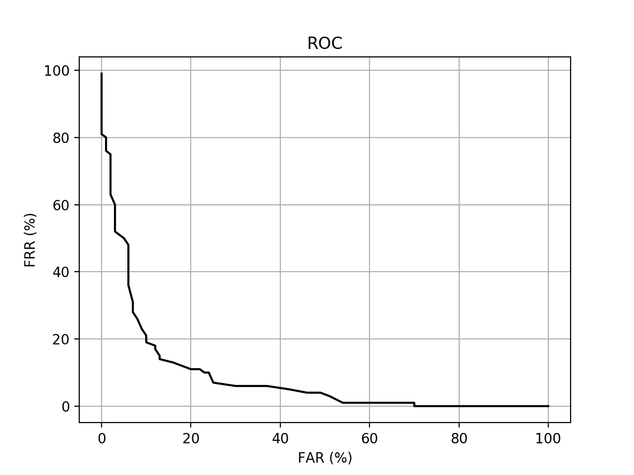
ROC
The Receiver Operating Characteristic (ROC) curve is one of the oldest plots in town. To plot an ROC curve, in possession of your negatives and positives, just do something along the lines of:
>>> from matplotlib import pyplot
>>> # we assume you have your negatives and positives already split
>>> npoints = 100
>>> bob.measure.plot.roc(negatives, positives, npoints, color=(0,0,0), linestyle='-', label='test')
>>> pyplot.xlabel('FAR (%)')
>>> pyplot.ylabel('FRR (%)')
>>> pyplot.grid(True)
>>> pyplot.show()
You should see an image like the following one:
(Source code, png, hires.png, pdf)

As can be observed, plotting methods live in the namespace
bob.measure.plot. They work like the
matplotlib.pyplot.plot() itself, except that instead of receiving the
x and y point coordinates as parameters, they receive the two
numpy.ndarray arrays with negatives and positives, as well as an
indication of the number of points the curve must contain.
As in the matplotlib.pyplot.plot() command, you can pass optional
parameters for the line as shown in the example to setup its color, shape and
even the label. For an overview of the keywords accepted, please refer to the
Matplotlib‘s Documentation. Other plot properties such as the plot title,
axis labels, grids, legends should be controlled directly using the relevant
Matplotlib‘s controls.
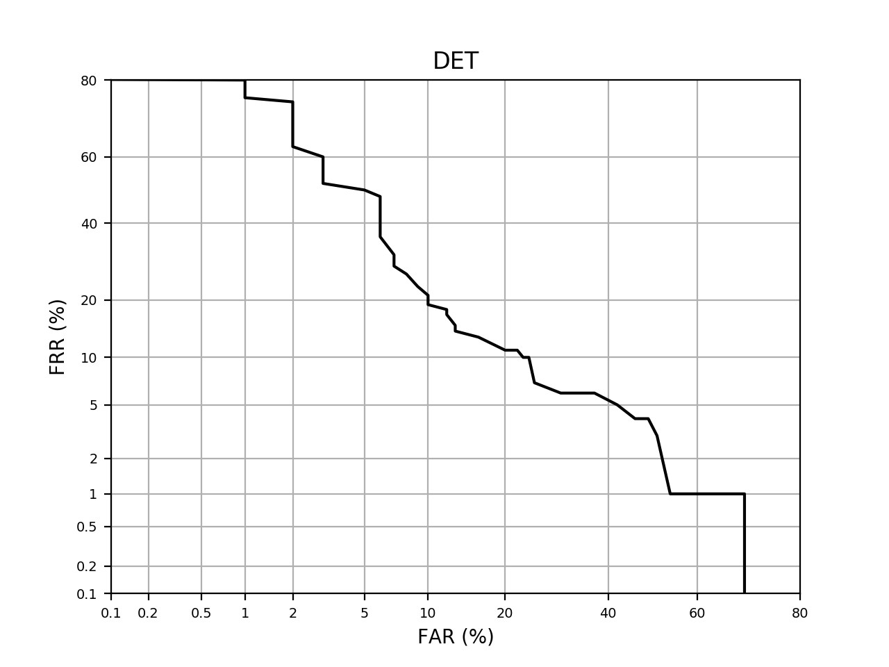
DET
A DET curve can be drawn using similar commands such as the ones for the ROC curve:
>>> from matplotlib import pyplot
>>> # we assume you have your negatives and positives already split
>>> npoints = 100
>>> bob.measure.plot.det(negatives, positives, npoints, color=(0,0,0), linestyle='-', label='test')
>>> bob.measure.plot.det_axis([0.01, 40, 0.01, 40])
>>> pyplot.xlabel('FAR (%)')
>>> pyplot.ylabel('FRR (%)')
>>> pyplot.grid(True)
>>> pyplot.show()
This will produce an image like the following one:
(Source code, png, hires.png, pdf)

Note
If you wish to reset axis zooming, you must use the Gaussian scale rather
than the visual marks showed at the plot, which are just there for
displaying purposes. The real axis scale is based on the
bob.measure.ppndf() method. For example, if you wish to set the x and y
axis to display data between 1% and 40% here is the recipe:
>>> #AFTER you plot the DET curve, just set the axis in this way:
>>> pyplot.axis([bob.measure.ppndf(k/100.0) for k in (1, 40, 1, 40)])
We provide a convenient way for you to do the above in this module. So,
optionally, you may use the bob.measure.plot.det_axis method like this:
>>> bob.measure.plot.det_axis([1, 40, 1, 40])
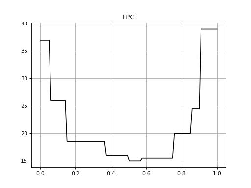
EPC
Drawing an EPC requires that both the development set negatives and positives are provided alongside the test (or evaluation) set ones. Because of this the API is slightly modified:
>>> bob.measure.plot.epc(dev_neg, dev_pos, test_neg, test_pos, npoints, color=(0,0,0), linestyle='-')
>>> pyplot.show()
This will produce an image like the following one:
(Source code, png, hires.png, pdf)
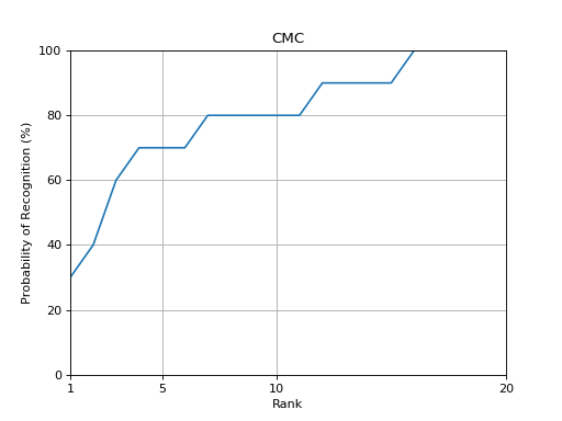
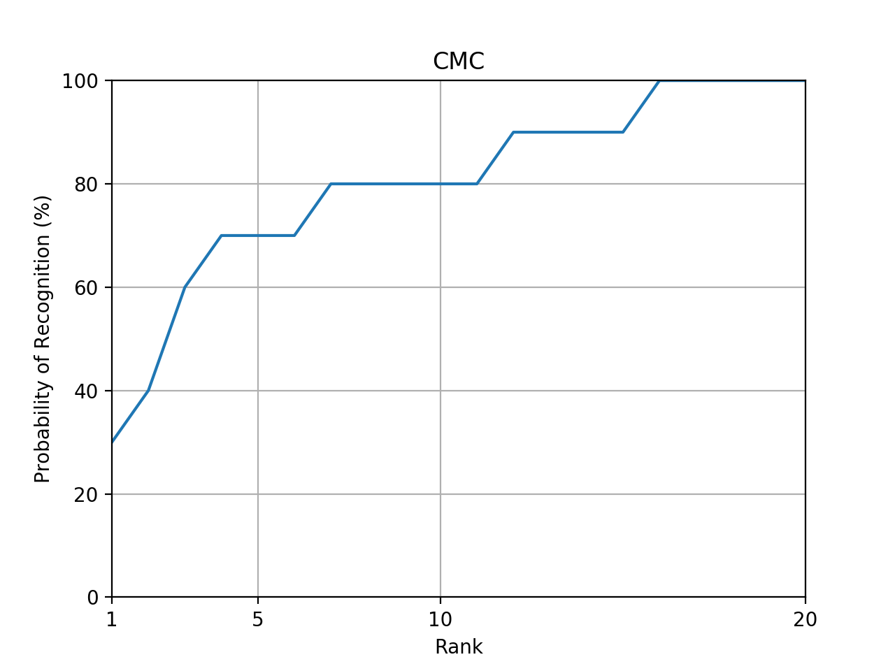
CMC
The Cumulative Match Characteristics (CMC) curve estimates the probability that
the correct model is in the N models with the highest similarity to a given
probe. A CMC curve can be plotted using the bob.measure.plot.cmc()
function. The CMC can be calculated from a relatively complex data structure,
which defines a pair of positive and negative scores per probe:
(Source code, png, hires.png, pdf)

Usually, there is only a single positive score per probe, but this is not a fixed restriction.
Note
The complex data structure can be read from our default 4 or 5 column score
files using the bob.measure.load.cmc_four_column() or
bob.measure.load.cmc_five_column() function.
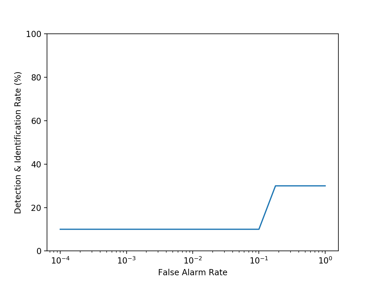
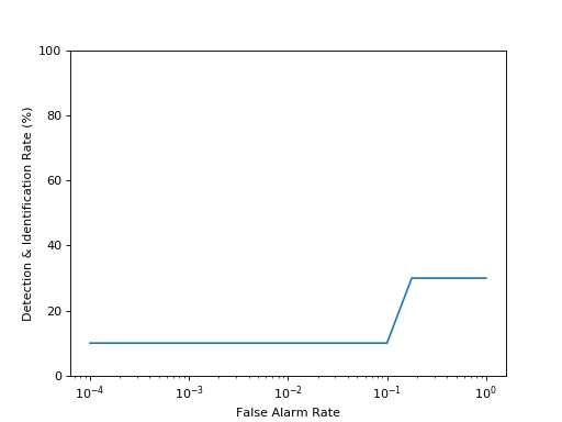
Detection & Identification Curve
The detection & identification curve is designed to evaluate open set
identification tasks. It can be plotted using the
bob.measure.plot.detection_identification_curve() function, but it
requires at least one open-set probe, i.e., where no corresponding positive
score exists, for which the FAR values are computed. Here, we plot the
detection and identification curve for rank 1, so that the recognition rate for
FAR=1 will be identical to the rank one bob.measure.recognition_rate()
obtained in the CMC plot above.
(Source code, png, hires.png, pdf)
Fine-tunning
The methods inside bob.measure.plot are only provided as a
Matplotlib wrapper to equivalent methods in bob.measure that can
only calculate the points without doing any plotting. You may prefer to tweak
the plotting or even use a different plotting system such as gnuplot. Have a
look at the implementations at bob.measure.plot to understand how to
use the Bob methods to compute the curves and interlace that in the way
that best suits you.
Full applications
We do provide a few scripts that can be used to quickly evaluate a set of
scores. We present these scripts in this section. The scripts take as input
either a 4-column or 5-column data format as specified in the documentation of
bob.measure.load.four_column() or
bob.measure.load.five_column().
To calculate the threshold using a certain criterion (EER, min.HTER or weighted Error Rate) on a set, after setting up Bob, just do:
$ bob_eval_threshold.py development-scores-4col.txt
Threshold: -0.004787956164
FAR : 6.731% (35/520)
FRR : 6.667% (26/390)
HTER: 6.699%
The output will present the threshold together with the FAR, FRR and HTER on the given set, calculated using such a threshold. The relative counts of FAs and FRs are also displayed between parenthesis.
To evaluate the performance of a new score file with a given threshold, use the
application bob_apply_threshold.py:
$ bob_apply_threshold.py -0.0047879 test-scores-4col.txt
FAR : 2.115% (11/520)
FRR : 7.179% (28/390)
HTER: 4.647%
In this case, only the error figures are presented. You can conduct the
evaluation and plotting of development (and test set data) using our combined
bob_compute_perf.py script. You pass both sets and it does the rest:
$ bob_compute_perf.py development-scores-4col.txt test-scores-4col.txt
[Min. criterion: EER] Threshold on Development set: -4.787956e-03
       | Development     | Test
-------+-----------------+------------------
  FAR  | 6.731% (35/520) | 2.500% (13/520)
  FRR  | 6.667% (26/390) | 6.154% (24/390)
  HTER | 6.699%          | 4.327%
[Min. criterion: Min. HTER] Threshold on Development set: 3.411070e-03
       | Development     | Test
-------+-----------------+------------------
  FAR  | 4.231% (22/520) | 1.923% (10/520)
  FRR  | 7.949% (31/390) | 7.692% (30/390)
  HTER | 6.090%          | 4.808%
[Plots] Performance curves => 'curves.pdf'
Inside that script we evaluate 2 different thresholds based on the EER and the minimum HTER on the development set and apply the output to the test set. As can be seen from the toy-example above, the system generalizes reasonably well. A single PDF file is generated containing an EPC as well as ROC and DET plots of such a system.
Use the --help option on the above-cited scripts to find-out about more
options.
Score file conversion
Sometimes, it is required to export the score files generated by Bob to a different format, e.g., to be able to generate a plot comparing Bob’s systems with other systems. In this package, we provide source code to convert between different types of score files.
Bob to OpenBR
One of the supported formats is the matrix format that the National Institute
of Standards and Technology (NIST) uses, and which is supported by OpenBR.
The scores are stored in two binary matrices, where the first matrix (usually
with a .mtx filename extension) contains the raw scores, while a second
mask matrix (extension .mask) contains information, which scores are
positives, and which are negatives.
To convert from Bob’s four column or five column score file to a pair of these
matrices, you can use the bob.measure.openbr.write_matrix() function.
In the simplest way, this function takes a score file
'five-column-sore-file' and writes the pair 'openbr.mtx', 'openbr.mask'
of OpenBR compatible files:
>>> bob.measure.openbr.write_matrix('five-column-sore-file', 'openbr.mtx', 'openbr.mask', score_file_format = '5column')
In this way, the score file will be parsed and the matrices will be written in the same order that is obtained from the score file.
For most of the applications, this should be sufficient, but as the identity
information is lost in the matrix files, no deeper analysis is possible anymore
when just using the matrices. To enforce an order of the models and probes
inside the matrices, you can use the model_names and probe_names
parameters of bob.measure.openbr.write_matrix():
The
probe_namesparameter lists thepathelements stored in the score files, which are the fourth column in a5columnfile, and the third column in a4columnfile, seebob.measure.load.five_column()andbob.measure.load.four_column().The
model_namesparameter is a bit more complicated. In a5columnformat score file, the model names are defined by the second column of that file, seebob.measure.load.five_column(). In a4columnformat score file, the model information is not contained, but only the client information of the model. Hence, for the4columnformat, themodel_namesactually lists the client ids found in the first column, seebob.measure.load.four_column().Warning
The model information is lost, but required to write the matrix files. In the
4columnformat, we use client ids instead of the model information. Hence, when several models exist per client, this function will not work as expected.
Additionally, there are fields in the matrix files, which define the gallery
and probe list files that were used to generate the matrix. These file names
can be selected with the gallery_file_name and probe_file_name keyword
parameters of bob.measure.openbr.write_matrix().
Finally, OpenBR defines a specific 'search' score file format, which is
designed to be used to compute CMC curves. The score matrix contains
descendingly sorted and possibly truncated list of scores, i.e., for each
probe, a sorted list of all scores for the models is generated. To generate
these special score file format, you can specify the search parameter. It
specifies the number of highest scores per probe that should be kept. If the
search parameter is set to a negative value, all scores will be kept. If
the search parameter is higher as the actual number of models, NaN
scores will be appended, and the according mask values will be set to 0
(i.e., to be ignored).
OpenBR to Bob
On the other hand, you might also want to generate a Bob-compatible (four or
five column) score file based on a pair of OpenBR matrix and mask files. This
is possible by using the bob.measure.openbr.write_score_file()
function. At the basic, it takes the given pair of matrix and mask files, as
well as the desired output score file:
>>> bob.measure.openbr.write_score_file('openbr.mtx', 'openbr.mask', 'four-column-sore-file')
This score file is sufficient to compute a CMC curve (see CMC), however it does not contain relevant client ids or paths for models and probes. Particularly, it assumes that each client has exactly one associated model.
To add/correct these information, you can use additional parameters to
bob.measure.openbr.write_score_file(). Client ids of models and
probes can be added using the models_ids and probes_ids keyword
arguments. The length of these lists must be identical to the number of models
and probes as given in the matrix files, and they must be in the same order
as used to compute the OpenBR matrix. This includes that the same
same-client and different-client pairs as indicated by the OpenBR mask will be
generated, which will be checked inside the function.
To add model and probe path information, the model_names and
probe_names parameters, which need to have the same size and order as the
models_ids and probes_ids. These information are simply stored in the
score file, and no further check is applied.
Note
The model_names parameter is used only when writing score files in score_file_format='5column', in the '4column' format, this parameter is ignored.