Python API
This section includes information for using the Python API of
bob.measure.
Measurement
Classification
bob.measure.correctly_classified_negatives(...) |
This method returns an array composed of booleans that pin-point, which |
bob.measure.correctly_classified_positives(...) |
This method returns an array composed of booleans that pin-point, which |
Single point measurements
bob.measure.farfrr((negatives, positives, ...) |
Calculates the false-acceptance (FA) ratio and the false-rejection (FR) |
bob.measure.f_score((negatives, positives, ...) |
This method computes the F-score of the accuracy of the classification |
bob.measure.precision_recall((negatives, ...) |
Calculates the precision and recall (sensitiveness) values given |
bob.measure.recognition_rate(cmc_scores[, ...]) |
Calculates the recognition rate from the given input |
bob.measure.detection_identification_rate(...) |
Computes the detection and identification rate for the given threshold. |
bob.measure.false_alarm_rate(cmc_scores, ...) |
Computes the false alarm rate for the given threshold,. |
bob.measure.eer_rocch((negatives, ...) |
Calculates the equal-error-rate (EER) given the input data, on the ROC |
Thresholds
bob.measure.eer_threshold((negatives, ...) |
Calculates the threshold that is as close as possible to the |
bob.measure.rocch2eer((pmiss_pfa) -> threshold) |
Calculates the threshold that is as close as possible to the |
bob.measure.min_hter_threshold((negatives, ...) |
Calculates the bob.measure.min_weighted_error_rate_threshold() |
bob.measure.min_weighted_error_rate_threshold(...) |
Calculates the threshold that minimizes the error rate for the given |
bob.measure.far_threshold((negatives, ...) |
Computes the threshold such that the real FAR is at least the |
bob.measure.frr_threshold((negatives, ...) |
Computes the threshold such that the real FRR is at least the |
Curves
bob.measure.roc((negatives, positives, ...) |
Calculates points of an Receiver Operating Characteristic (ROC) |
bob.measure.rocch((negatives, ...) |
Calculates the ROC Convex Hull (ROCCH) curve given a set of positive |
bob.measure.roc_for_far((negatives, ...) |
Calculates the ROC curve for a given set of positive and negative |
bob.measure.det((negatives, positives, ...) |
Calculates points of an Detection Error-Tradeoff (DET) curve |
bob.measure.epc((dev_negatives, ...) |
Calculates points of an Expected Performance Curve (EPC) |
bob.measure.precision_recall_curve(...) |
Calculates the precision-recall curve given a set of positive and |
bob.measure.cmc(cmc_scores) |
Calculates the cumulative match characteristic (CMC) from the given input. |
Generic
bob.measure.ppndf((value) -> ppndf) |
Returns the Deviate Scale equivalent of a false rejection/acceptance |
bob.measure.relevance(input, machine) |
Calculates the relevance of every input feature to the estimation process |
bob.measure.mse(estimation, target) |
Mean square error between a set of outputs and target values |
bob.measure.rmse(estimation, target) |
Calculates the root mean square error between a set of outputs and target |
bob.measure.get_config() |
Returns a string containing the configuration information. |
Loading data
bob.measure.load.open_file(filename[, mode]) |
Opens the given score file for reading. |
bob.measure.load.four_column(filename) |
Loads a score set from a single file and yield its lines |
bob.measure.load.split_four_column(filename) |
Loads a score set from a single file and splits the scores |
bob.measure.load.cmc_four_column(filename) |
Loads scores to compute CMC curves from a file in four column format. |
bob.measure.load.five_column(filename) |
Loads a score set from a single file and yield its lines |
bob.measure.load.split_five_column(filename) |
Loads a score set from a single file and splits the scores |
bob.measure.load.cmc_five_column(filename) |
Loads scores to compute CMC curves from a file in five column format. |
Calibration
bob.measure.calibration.cllr(negatives, ...) |
Cost of log likelihood ratio as defined by the Bosaris toolkit |
bob.measure.calibration.min_cllr(negatives, ...) |
Minimum cost of log likelihood ratio as defined by the Bosaris toolkit |
Plotting
bob.measure.plot.roc(negatives, positives[, ...]) |
Plots Receiver Operating Characteristic (ROC) curve. |
bob.measure.plot.det(negatives, positives[, ...]) |
Plots Detection Error Trade-off (DET) curve as defined in the paper: |
bob.measure.plot.det_axis(v, **kwargs) |
Sets the axis in a DET plot. |
bob.measure.plot.epc(dev_negatives, ...[, ...]) |
Plots Expected Performance Curve (EPC) as defined in the paper: |
bob.measure.plot.precision_recall_curve(...) |
Plots a Precision-Recall curve. |
bob.measure.plot.cmc(cmc_scores[, logx]) |
Plots the (cumulative) match characteristics and returns the maximum rank. |
bob.measure.plot.detection_identification_curve(...) |
Plots the Detection & Identification curve over the FAR |
OpenBR conversions
bob.measure.openbr.write_matrix(score_file, ...) |
Writes the OpenBR matrix and mask files (version 2), given a score file. |
bob.measure.openbr.write_score_file(...[, ...]) |
Writes the Bob score file in the desired format from OpenBR files. |
Details
-
bob.measure.mse(estimation, target)[source]¶ Mean square error between a set of outputs and target values
Uses the formula:
![MSE(\hat{\Theta}) = E[(\hat{\Theta} - \Theta)^2]](../../../_images/math/806819950757f705fabed699a1e754545e22f36e.png)
Estimation (
 ) and target (
 ) are supposed to
have 2 dimensions. Different examples are organized as rows while different
features in the estimated values or targets are organized as different
columns.
) are supposed to
have 2 dimensions. Different examples are organized as rows while different
features in the estimated values or targets are organized as different
columns.Parameters:
- estimation (array): an N-dimensional array that corresponds to the value
- estimated by your procedure
- target (array): an N-dimensional array that corresponds to the expected
- value
Returns:
float: The average of the squared error between the estimated value and the target
-
bob.measure.rmse(estimation, target)[source]¶ Calculates the root mean square error between a set of outputs and target
Uses the formula:
![RMSE(\hat{\Theta}) = \sqrt(E[(\hat{\Theta} - \Theta)^2])](../../../_images/math/9f3c6c2293e8f70ca15eb41d89601bb1f6a58aca.png)
Estimation (
) and target () are supposed to
have 2 dimensions. Different examples are organized as rows while different
features in the estimated values or targets are organized as different
columns.Parameters:
- estimation (array): an N-dimensional array that corresponds to the value
- estimated by your procedure
- target (array): an N-dimensional array that corresponds to the expected
- value
Returns:
float: The square-root of the average of the squared error between the estimated value and the target
-
bob.measure.relevance(input, machine)[source]¶ Calculates the relevance of every input feature to the estimation process
Uses the formula:
Neural Triggering System Operating on High Resolution Calorimetry Information, Anjos et al, April 2006, Nuclear Instruments and Methods in Physics Research, volume 559, pages 134-138![R(x_{i}) = |E[(o(x) - o(x|x_{i}=E[x_{i}]))^2]|](../../../_images/math/7f8159bbf686612ed1c272cb44c97e1c78d0b0cc.png)
In other words, the relevance of a certain input feature i is the change on the machine output value when such feature is replaced by its mean for all input vectors. For this to work, the input parameter has to be a 2D array with features arranged column-wise while different examples are arranged row-wise.
Parameters:
- input (array): an N-dimensional array that corresponds to the value
- estimated by your model
machine (object): A machine that can be called to “process” your input
Returns:
array: An 1D float array as large as the number of columns (second dimension) of your input array, estimating the “relevance” of each input column (or feature) to the score provided by the machine.
-
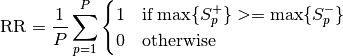
bob.measure.recognition_rate(cmc_scores, threshold=None, rank=1)[source]¶ Calculates the recognition rate from the given input
It is identical to the CMC value for the given
rank.The input has a specific format, which is a list of two-element tuples. Each of the tuples contains the negative
 and the positive
 scores for one probe item
  , or
, or Nonein case of open set recognition. To read the lists from score files in 4 or 5 column format, please use thebob.measure.load.cmc_four_column()orbob.measure.load.cmc_five_column()function.If
thresholdis set toNone, the rank 1 recognition rate is defined as the number of test items, for which the highest positive score is greater than or equal to all negative
scores, divided by the number of all probe items
score is greater than or equal to all negative
scores, divided by the number of all probe items  :
:
For a given rank
 , up to
  negative scores that are higher
than the highest positive score are allowed to still count as correctly
classified in the top rank.
negative scores that are higher
than the highest positive score are allowed to still count as correctly
classified in the top rank.If
threshold is given, all scores below threshold
will be filtered out. Hence, if all positive scores are below threshold
is given, all scores below threshold
will be filtered out. Hence, if all positive scores are below threshold
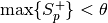 , the probe will be misclassified at any
rank.
, the probe will be misclassified at any
rank.For open set recognition, i.e., when there exist a tuple including negative scores without corresponding positive scores (
None), and all negative scores are belowthreshold, the probe
item is correctly rejected, and it does not count into the denominator
. When no thresholdis provided, the open set probes will always count as misclassified, regardless of therank.Parameters:
- cmc_scores (list): A list in the format
[(negatives, positives), ...] containing the CMC scores loaded with one of the functions (
bob.measure.load.cmc_four_column()orbob.measure.load.cmc_five_column()).Each pair contains the
negativeand thepositivescores for one probe item. Each pair can contain up to one empty array (orNone), i.e., in case of open set recognition.- threshold (
float, optional): Decision threshold. If notNone, all - scores will be filtered by the threshold. In an open set recognition problem, all open set scores (negatives with no corresponding positive) for which all scores are below threshold, will be counted as correctly rejected and removed from the probe list (i.e., the denominator).
- rank (
int, optional): - The rank for which the recognition rate should be computed, 1 by default.
Returns:
float: The (open set) recognition rate for the given rank, a value between 0 and 1.- cmc_scores (list): A list in the format
-
bob.measure.cmc(cmc_scores)[source]¶ Calculates the cumulative match characteristic (CMC) from the given input.
The input has a specific format, which is a list of two-element tuples. Each of the tuples contains the negative and the positive scores for one probe item. To read the lists from score files in 4 or 5 column format, please use the
bob.measure.load.cmc_four_column()orbob.measure.load.cmc_five_column()function.For each probe item the probability that the rank
of the positive
score is calculated. The rank is computed as the number of negative scores
that are higher than the positive score. If several positive scores for one
test item exist, the highest positive score is taken. The CMC finally
computes how many test items have rank r or higher, divided by the total
number of test values.Note
The CMC is not available for open set classification. Please use the
detection_identification_rate()andfalse_alarm_rate()instead.Parameters:
- cmc_scores (list): A list in the format
[(negatives, positives), ...] containing the CMC scores loaded with one of the functions (
bob.measure.load.cmc_four_column()orbob.measure.load.cmc_five_column()).Each pair contains the
negativeand thepositivescores for one probe item. Each pair can contain up to one empty array (orNone), i.e., in case of open set recognition.
Returns:
array: A 2D float array representing the CMC curve, with the Rank in the first column and the number of correctly classified clients (in this rank) in the second column.- cmc_scores (list): A list in the format
-
bob.measure.detection_identification_rate(cmc_scores, threshold, rank=1)[source]¶ Computes the detection and identification rate for the given threshold.
This value is designed to be used in an open set identification protocol, and defined in Chapter 14.1 of [LiJain2005].
Although the detection and identification rate is designed to be computed on an open set protocol, it uses only the probe elements, for which a corresponding gallery element exists. For closed set identification protocols, this function is identical to
recognition_rate(). The only difference is that for this function, athresholdfor the scores need to be defined, while forrecognition_rate()it is optional.Parameters:
- cmc_scores (list): A list in the format
[(negatives, positives), ...] containing the CMC scores loaded with one of the functions (
bob.measure.load.cmc_four_column()orbob.measure.load.cmc_five_column()).Each pair contains the
negativeand thepositivescores for one probe item. Each pair can contain up to one empty array (orNone), i.e., in case of open set recognition.
threshold (float): The decision threshold
 .
.rank (
int, optional): The rank for which the curve should be plottedReturns:
float: The detection and identification rate for the given threshold.- cmc_scores (list): A list in the format
-
bob.measure.false_alarm_rate(cmc_scores, threshold)[source]¶ Computes the false alarm rate for the given threshold,.
This value is designed to be used in an open set identification protocol, and defined in Chapter 14.1 of [LiJain2005].
The false alarm rate is designed to be computed on an open set protocol, it uses only the probe elements, for which no corresponding gallery element exists.
Parameters:
- cmc_scores (list): A list in the format
[(negatives, positives), ...] containing the CMC scores loaded with one of the functions (
bob.measure.load.cmc_four_column()orbob.measure.load.cmc_five_column()).Each pair contains the
negativeand thepositivescores for one probe item. Each pair can contain up to one empty array (orNone), i.e., in case of open set recognition.
threshold (float): The decision threshold
.Returns:
float: The false alarm rate.- cmc_scores (list): A list in the format
-
bob.measure.correctly_classified_negatives(negatives, threshold) → classified¶ This method returns an array composed of booleans that pin-point, which negatives where correctly classified for the given threshold
The pseudo-code for this function is:
foreach (k in negatives) if negatives[k] < threshold: classified[k]
= true else: classified[k] = false
Parameters:
negatives: array_like(1D, float)The scores generated by comparing objects of different classesthreshold: floatThe threshold, for which scores should be considered to be correctly classifiedReturns:
classified: array_like(1D, bool)The decision for each of thenegatives
-
bob.measure.correctly_classified_positives(positives, threshold) → classified¶ This method returns an array composed of booleans that pin-point, which positives where correctly classified for the given threshold
The pseudo-code for this function is:
foreach (k in positives) if positives[k] >= threshold:
classified[k] = true else: classified[k] = false
Parameters:
positives: array_like(1D, float)The scores generated by comparing objects of the same classesthreshold: floatThe threshold, for which scores should be considered to be correctly classifiedReturns:
classified: array_like(1D, bool)The decision for each of thepositives
-
bob.measure.det(negatives, positives, n_points) → curve¶ Calculates points of an Detection Error-Tradeoff (DET) curve
Calculates the DET curve given a set of negative and positive scores and a desired number of points. Returns a two-dimensional array of doubles that express on its rows:
[0] X axis values in the normal deviate scale for the false-accepts
[1] Y axis values in the normal deviate scale for the false-rejections
You can plot the results using your preferred tool to first create a plot using rows 0 and 1 from the returned value and then replace the X/Y axis annotation using a pre-determined set of tickmarks as recommended by NIST. The derivative scales are computed with the
bob.measure.ppndf()function.Parameters:
negatives, positives: array_like(1D, float)The list of negative and positive scores to compute the DET forn_points: intThe number of points on the DET curve, for which the DET should be evaluatedReturns:
curve: array_like(2D, float)The DET curve, with the FAR in the first and the FRR in the second row
-
bob.measure.eer_rocch(negatives, positives) → threshold¶ Calculates the equal-error-rate (EER) given the input data, on the ROC Convex Hull (ROCCH)
It replicates the EER calculation from the Bosaris toolkit (https://sites.google.com/site/bosaristoolkit/).
Parameters:
negatives, positives: array_like(1D, float)The set of negative and positive scores to compute the thresholdReturns:
threshold: floatThe threshold for the equal error rate
-
bob.measure.eer_threshold(negatives, positives[, is_sorted]) → threshold¶ Calculates the threshold that is as close as possible to the equal-error-rate (EER) for the given input data
The EER should be the point where the FAR equals the FRR. Graphically, this would be equivalent to the intersection between the ROC (or DET) curves and the identity.
Note
The scores will be sorted internally, requiring the scores to be copied. To avoid this copy, you can sort both sets of scores externally in ascendant order, and set the
is_sortedparameter toTrueParameters:
negatives, positives: array_like(1D, float)The set of negative and positive scores to compute the thresholdis_sorted: bool[Default:False] Are both sets of scores already in ascendantly sorted order?Returns:
threshold: floatThe threshold (i.e., as used inbob.measure.farfrr()) where FAR and FRR are as close as possible
-
bob.measure.epc(dev_negatives, dev_positives, test_negatives, test_positives, n_points, is_sorted) → curve¶ Calculates points of an Expected Performance Curve (EPC)
Calculates the EPC curve given a set of positive and negative scores and a desired number of points. Returns a two-dimensional
numpy.ndarrayof type float that express the X (cost) and Y (weighted error rare on the test set given the min. threshold on the development set) coordinates in this order. Please note that, in order to calculate the EPC curve, one needs two sets of data comprising a development set and a test set. The minimum weighted error is calculated on the development set and then applied to the test set to evaluate the weighted error rate at that position.The EPC curve plots the HTER on the test set for various values of ‘cost’. For each value of ‘cost’, a threshold is found that provides the minimum weighted error (see
bob.measure.min_weighted_error_rate_threshold()) on the development set. Each threshold is consecutively applied to the test set and the resulting weighted error values are plotted in the EPC.The cost points in which the EPC curve are calculated are distributed uniformly in the range
![[0.0, 1.0]](../../../_images/math/a7641574e45d541f49c7eaa2b29080712d499327.png) .
.Note
It is more memory efficient, when sorted arrays of scores are provided and the
is_sortedparameter is set toTrue.Parameters:
dev_negatives, dev_positives, test_negatives, test_positives: array_like(1D, float)The scores for negatives and positives of the development and test setn_points: intThe number of weights for which the EPC curve should be computedis_sorted: bool[Default:False] Set this toTrueif the scores are already sorted. IfFalse, scores will be sorted internally, which will require more memoryReturns:
curve: array_like(2D, float)The EPC curve, with the first row containing the weights, and the second row containing the weighted thresholds on the test set
-
bob.measure.f_score(negatives, positives, threshold[, weight]) → f_score¶ This method computes the F-score of the accuracy of the classification
The F-score is a weighted mean of precision and recall measurements, see
bob.measure.precision_recall(). It is computed as: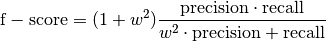
The weight
 needs to be non-negative real value. In case the
weight parameter is 1 (the default), the F-score is called F1 score and
is a harmonic mean between precision and recall values.
needs to be non-negative real value. In case the
weight parameter is 1 (the default), the F-score is called F1 score and
is a harmonic mean between precision and recall values.Parameters:
negatives, positives: array_like(1D, float)The set of negative and positive scores to compute the precision and recallthreshold: floatThe threshold to compute the precision and recall forweight: float[Default:1] The weight between precision and recallReturns:
f_score: floatThe computed f-score for the given scores and the given threshold
-
bob.measure.far_threshold(negatives, positives[, far_value][, is_sorted]) → threshold¶ Computes the threshold such that the real FAR is at least the requested
far_valueNote
The scores will be sorted internally, requiring the scores to be copied. To avoid this copy, you can sort the
negativesscores externally in ascendant order, and set theis_sortedparameter toTrueParameters:
negatives: array_like(1D, float)The set of negative scores to compute the FAR thresholdpositives: array_like(1D, float)Ignored, but needs to be specified – may be given as[]far_value: float[Default:0.001] The FAR value, for which the threshold should be computedis_sorted: bool[Default:False] Set this toTrueif thenegativesare already sorted in ascending order. IfFalse, scores will be sorted internally, which will require more memoryReturns:
threshold: floatThe threshold such that the real FAR is at leastfar_value
-
bob.measure.farfrr(negatives, positives, threshold) → far, frr¶ Calculates the false-acceptance (FA) ratio and the false-rejection (FR) ratio for the given positive and negative scores and a score threshold
positivesholds the score information for samples that are labeled to belong to a certain class (a.k.a., ‘signal’ or ‘client’).negativesholds the score information for samples that are labeled not to belong to the class (a.k.a., ‘noise’ or ‘impostor’). It is expected that ‘positive’ scores are, at least by design, greater than ‘negative’ scores. So, every ‘positive’ value that falls bellow the threshold is considered a false-rejection (FR). negative samples that fall above the threshold are considered a false-accept (FA).Positives that fall on the threshold (exactly) are considered correctly classified. Negatives that fall on the threshold (exactly) are considered incorrectly classified. This equivalent to setting the comparison like this pseudo-code:
foreach (positive as K) if K < threshold: falseRejectionCount +=
1
foreach (negative as K) if K >= threshold: falseAcceptCount += 1The output is in form of a tuple of two double-precision real numbers. The numbers range from 0 to 1. The first element of the pair is the false-accept ratio (FAR), the second element the false-rejection ratio (FRR).
The
thresholdvalue does not necessarily have to fall in the range covered by the input scores (negatives and positives altogether), but if it does not, the output will be either (1.0, 0.0) or (0.0, 1.0), depending on the side the threshold falls.It is possible that scores are inverted in the negative/positive sense. In some setups the designer may have setup the system so ‘positive’ samples have a smaller score than the ‘negative’ ones. In this case, make sure you normalize the scores so positive samples have greater scores before feeding them into this method.
Parameters:
negatives: array_like(1D, float)The scores for comparisons of objects of different classespositives: array_like(1D, float)The scores for comparisons of objects of the same classthreshold: floatThe threshold to separate correctly and incorrectly classified scoresReturns:
far: floatThe False Accept Rate (FAR) for the given thresholdfrr: floatThe False Reject Rate (FRR) for the given threshold
-
bob.measure.frr_threshold(negatives, positives[, frr_value][, is_sorted]) → threshold¶ Computes the threshold such that the real FRR is at least the requested
frr_valueNote
The scores will be sorted internally, requiring the scores to be copied. To avoid this copy, you can sort the
positivesscores externally in ascendant order, and set theis_sortedparameter toTrueParameters:
negatives: array_like(1D, float)Ignored, but needs to be specified – may be given as[]positives: array_like(1D, float)The set of positive scores to compute the FRR thresholdfrr_value: float[Default:0.001] The FRR value, for which the threshold should be computedis_sorted: bool[Default:False] Set this toTrueif thepositivesare already sorted in ascendant order. IfFalse, scores will be sorted internally, which will require more memoryReturns:
threshold: floatThe threshold such that the real FRR is at leastfrr_value
-
bob.measure.min_hter_threshold(negatives, positives[, is_sorted]) → threshold¶ Calculates the
bob.measure.min_weighted_error_rate_threshold()withcost=0.5Parameters:
negatives, positives: array_like(1D, float)The set of negative and positive scores to compute the thresholdis_sorted: bool[Default:False] Are both sets of scores already in ascendantly sorted order?Returns:
threshold: floatThe threshold for which the weighted error rate is minimal
-
bob.measure.min_weighted_error_rate_threshold(negatives, positives, cost[, is_sorted]) → threshold¶ Calculates the threshold that minimizes the error rate for the given input data
The
costparameter determines the relative importance between false-accepts and false-rejections. This number should be between 0 and 1 and will be clipped to those extremes. The value to minimize becomes: . The higher the cost,
the higher the importance given to not making mistakes classifying
negatives/noise/impostors.
. The higher the cost,
the higher the importance given to not making mistakes classifying
negatives/noise/impostors.Note
The scores will be sorted internally, requiring the scores to be copied. To avoid this copy, you can sort both sets of scores externally in ascendant order, and set the
is_sortedparameter toTrueParameters:
negatives, positives: array_like(1D, float)The set of negative and positive scores to compute the thresholdcost: floatThe relative cost over FAR with respect to FRR in the threshold calculationis_sorted: bool[Default:False] Are both sets of scores already in ascendantly sorted order?Returns:
threshold: floatThe threshold for which the weighted error rate is minimal
-
bob.measure.ppndf(value) → ppndf¶ Returns the Deviate Scale equivalent of a false rejection/acceptance ratio
The algorithm that calculates the deviate scale is based on function ppndf() from the NIST package DETware version 2.1, freely available on the internet. Please consult it for more details. By 20.04.2011, you could find such package here.
Parameters:
value: floatThe value (usually FAR or FRR) for which the ppndf should be calculatedReturns:
ppndf: floatThe derivative scale of the given value
-
bob.measure.precision_recall(negatives, positives, threshold) → precision, recall¶ Calculates the precision and recall (sensitiveness) values given negative and positive scores and a threshold
Precision and recall are computed as:
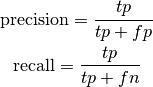
where
 are the true positives,
  are the false
positives and
are the false
positives and  are the false negatives.
positivesholds the score information for samples that are labeled to belong to a certain class (a.k.a., ‘signal’ or ‘client’).negativesholds the score information for samples that are labeled not to belong to the class (a.k.a., ‘noise’ or ‘impostor’). For more precise details about how the method considers error rates, seebob.measure.farfrr().Parameters:
negatives, positives: array_like(1D, float)The set of negative and positive scores to compute the measurementsthreshold: floatThe threshold to compute the measures forReturns:
precision: floatThe precision value for the given negatives and positivesrecall: floatThe recall value for the given negatives and positives
-
bob.measure.precision_recall_curve(negatives, positives, n_points) → curve¶ Calculates the precision-recall curve given a set of positive and negative scores and a number of desired points
The points in which the curve is calculated are distributed uniformly in the range
[min(negatives, positives), max(negatives, positives)]Parameters:
negatives, positives: array_like(1D, float)The set of negative and positive scores to compute the measurementsn_points: intThe number of thresholds for which precision and recall should be evaluatedReturns:
curve: array_like(2D, float)- 2D array of floats that express the X (precision) and Y (recall)
- coordinates
-
bob.measure.roc(negatives, positives, n_points) → curve¶ Calculates points of an Receiver Operating Characteristic (ROC)
Calculates the ROC curve given a set of negative and positive scores and a desired number of points.
Parameters:
negatives, positives: array_like(1D, float)The negative and positive scores, for which the ROC curve should be calculatedn_points: intThe number of points, in which the ROC curve are calculated, which are distributed uniformly in the range[min(negatives, positives), max(negatives, positives)]Returns:
curve: array_like(2D, float)A two-dimensional array of doubles that express the X (FAR) and Y (FRR) coordinates in this order
-
bob.measure.roc_for_far(negatives, positives, far_list[, is_sorted]) → curve¶ Calculates the ROC curve for a given set of positive and negative scores and the FAR values, for which the FRR should be computed
Note
The scores will be sorted internally, requiring the scores to be copied. To avoid this copy, you can sort both sets of scores externally in ascendant order, and set the
is_sortedparameter toTrueParameters:
negatives, positives: array_like(1D, float)The set of negative and positive scores to compute the curvefar_list: array_like(1D, float)A list of FAR values, for which the FRR values should be computedis_sorted: bool[Default:False] Set this toTrueif both sets of scores are already sorted in ascending order. IfFalse, scores will be sorted internally, which will require more memoryReturns:
curve: array_like(2D, float)The ROC curve, which holds a copy of the given FAR values in row 0, and the corresponding FRR values in row 1
-
bob.measure.rocch(negatives, positives) → curve¶ Calculates the ROC Convex Hull (ROCCH) curve given a set of positive and negative scores
Parameters:
negatives, positives: array_like(1D, float)The set of negative and positive scores to compute the curveReturns:
curve: array_like(2D, float)The ROC curve, with the first row containing the FAR, and the second row containing the FRR
-
bob.measure.rocch2eer(pmiss_pfa) → threshold¶ Calculates the threshold that is as close as possible to the equal-error-rate (EER) given the input data
Returns:
threshold: floatThe computed threshold, at which the EER can be obtained
A set of utilities to load score files with different formats.
-
bob.measure.load.open_file(filename, mode='rt')[source]¶ Opens the given score file for reading.
Score files might be raw text files, or a tar-file including a single score file inside.
Parameters:
- filename (
str,file-like): The name of the score file to - open, or a file-like object open for reading. If a file name is given, the according file might be a raw text file or a (compressed) tar file containing a raw text file.
Returns:
file-like: A read-only file-like object as it would be returned byopen().- filename (
-
bob.measure.load.four_column(filename)[source]¶ Loads a score set from a single file and yield its lines
Loads a score set from a single file and yield its lines (to avoid loading the score file at once into memory). This function verifies that all fields are correctly placed and contain valid fields. The score file must contain the following information in each line:
claimed_id real_id test_label score
Parameters:
- filename (
str,file-like): The file object that will be - opened with
open_file()containing the scores.
Returns:
str: The claimed identity – the client name of the model that was used in the comparison
str: The real identity – the client name of the probe that was used in the comparison
str: A label of the probe – usually the probe file name, or the probe id
float: The result of the comparison of the model and the probe
- filename (
-
bob.measure.load.split_four_column(filename)[source]¶ Loads a score set from a single file and splits the scores
Loads a score set from a single file and splits the scores between negatives and positives. The score file has to respect the 4 column format as defined in the method
four_column().This method avoids loading and allocating memory for the strings present in the file. We only keep the scores.
Parameters:
- filename (
str,file-like): The file object that will be - opened with
open_file()containing the scores.
Returns:
negatives (array): 1D float array containing the list of scores, for which the
claimed_idand thereal_iddiffered (seefour_column())positivies (array): 1D float array containing the list of scores, for which the
claimed_idand thereal_idare identical (seefour_column())- filename (
-
bob.measure.load.cmc_four_column(filename)[source]¶ Loads scores to compute CMC curves from a file in four column format.
The four column file needs to be in the same format as described in
four_column(), and thetest_label(column 3) has to contain the test/probe file name or a probe id.This function returns a list of tuples. For each probe file, the tuple consists of a list of negative scores and a list of positive scores. Usually, the list of positive scores should contain only one element, but more are allowed. The result of this function can directly be passed to, e.g., the
bob.measure.cmc()function.Parameters:
- filename (
str,file-like): The file object that will be - opened with
open_file()containing the scores.
Returns:
list: A list of tuples, where each tuple contains thenegativeandpositivescores for one probe of the database. Bothnegativesandpositivescan be either an 1Dnumpy.ndarrayof typefloat, orNone.- filename (
-
bob.measure.load.five_column(filename)[source]¶ Loads a score set from a single file and yield its lines
Loads a score set from a single file and yield its lines (to avoid loading the score file at once into memory). This function verifies that all fields are correctly placed and contain valid fields. The score file must contain the following information in each line:
claimed_id model_label real_id test_label score
Parameters:
- filename (
str,file-like): The file object that will be - opened with
open_file()containing the scores.
Returns:
str: The claimed identity – the client name of the model that was used in the comparison
str: A label for the model – usually the model file name, or the model id
str: The real identity – the client name of the probe that was used in the comparison
str: A label of the probe – usually the probe file name, or the probe id
float: The result of the comparison of the model and the probe
- filename (
-
bob.measure.load.split_five_column(filename)[source]¶ Loads a score set from a single file and splits the scores
Loads a score set from a single file in five column format and splits the scores between negatives and positives. The score file has to respect the 5 column format as defined in the method
five_column().This method avoids loading and allocating memory for the strings present in the file. We only keep the scores.
Parameters:
- filename (
str,file-like): The file object that will be - opened with
open_file()containing the scores.
Returns:
negatives (array): 1D float array containing the list of scores, for which the
claimed_idand thereal_iddiffered (seefour_column())positivies (array): 1D float array containing the list of scores, for which the
claimed_idand thereal_idare identical (seefour_column())- filename (
-
bob.measure.load.cmc_five_column(filename)[source]¶ Loads scores to compute CMC curves from a file in five column format.
The five column file needs to be in the same format as described in
five_column(), and thetest_label(column 4) has to contain the test/probe file name or a probe id.This function returns a list of tuples. For each probe file, the tuple consists of a list of negative scores and a list of positive scores. Usually, the list of positive scores should contain only one element, but more are allowed. The result of this function can directly be passed to, e.g., the
bob.measure.cmc()function.Parameters:
- filename (
str,file-like): The file object that will be - opened with
open_file()containing the scores.
Returns:
list: A list of tuples, where each tuple contains thenegativeandpositivescores for one probe of the database.- filename (
-
bob.measure.load.load_score(filename, ncolumns=None)[source]¶ Load scores using numpy.loadtxt and return the data as a numpy array.
Parameters:
- filename (
str,file-like): The file object that will be - opened with
open_file()containing the scores. - ncolumns (
int, optional): 4, 5 or None (the default), - specifying the number of columns in the score file. If None is provided, the number of columns will be guessed.
Returns:
array: An array which contains not only the actual scores but also theclaimed_id,real_id,test_labeland['model_label']- filename (
-
bob.measure.load.get_negatives_positives(score_lines)[source]¶ Take the output of load_score and return negatives and positives. This function aims to replace split_four_column and split_five_column but takes a different input. It’s up to you to use which one.
-
bob.measure.load.get_negatives_positives_all(score_lines_list)[source]¶ Take a list of outputs of load_score and return stacked negatives and positives.
-
bob.measure.load.get_all_scores(score_lines_list)[source]¶ Take a list of outputs of load_score and return stacked scores
-
bob.measure.load.dump_score(filename, score_lines)[source]¶ Dump scores that were loaded using
load_score()The number of columns is automatically detected.
Measures for calibration
-
bob.measure.calibration.cllr(negatives, positives)[source]¶ Cost of log likelihood ratio as defined by the Bosaris toolkit
Computes the ‘cost of log likelihood ratio’ (
 ) measure as
given in the Bosaris toolkit
) measure as
given in the Bosaris toolkitParameters:
- negatives (array): 1D float array that contains the scores of the
- “negative” (noise, non-class) samples of your classifier.
- positives (array): 1D float array that contains the scores of the
- “positive” (signal, class) samples of your classifier.
Returns:
float: The computed value.
-
bob.measure.calibration.min_cllr(negatives, positives)[source]¶ Minimum cost of log likelihood ratio as defined by the Bosaris toolkit
Computes the ‘minimum cost of log likelihood ratio’ (
 )
measure as given in the bosaris toolkit
)
measure as given in the bosaris toolkitParameters:
- negatives (array): 1D float array that contains the scores of the
- “negative” (noise, non-class) samples of your classifier.
- positives (array): 1D float array that contains the scores of the
- “positive” (signal, class) samples of your classifier.
Returns:
float: The computed value.
-
bob.measure.plot.log_values(min_step=-4, counts_per_step=4)[source]¶ Computes log-scaled values between
 and 1
and 1This function computes log-scaled values between
and 1
(including), where  is the
 min_steargument, which needs to be a negative integer. The integralcounts_per_stepvalue defines how many values between two adjacent powers of 10 will be created. The total number of values will be-min_step * counts_per_step + 1.Parameters:
- min_step (
int, optional): The power of 10 that will be the - minimum value. E.g., the default
-4will result in the first number to be =
= 0.00001or0.01% - counts_per_step (
int, optional): The number of values that will - be put between two adjacent powers of 10. With the default value
4(and default values ofmin_step), we will getlog_list[0] == 1e-4,log_list[4] == 1e-3, ...,log_list[16] == 1.
Returns:
list: A list of logarithmically scaled values between and 1.- min_step (
-
bob.measure.plot.roc(negatives, positives, npoints=100, CAR=False, **kwargs)[source]¶ Plots Receiver Operating Characteristic (ROC) curve.
This method will call
matplotlibto plot the ROC curve for a system which contains a particular set of negatives (impostors) and positives (clients) scores. We use the standardmatplotlib.pyplot.plot()command. All parameters passed with exception of the three first parameters of this method will be directly passed to the plot command.The plot will represent the false-alarm on the horizontal axis and the false-rejection on the vertical axis. The values for the axis will be computed using
bob.measure.roc().Note
This function does not initiate and save the figure instance, it only issues the plotting command. You are the responsible for setting up and saving the figure as you see fit.
Parameters:
- negatives (array): 1D float array that contains the scores of the
- “negative” (noise, non-class) samples of your classifier. See
(
bob.measure.roc()) - positives (array): 1D float array that contains the scores of the
- “positive” (signal, class) samples of your classifier. See
(
bob.measure.roc()) - npoints (
int, optional): The number of points for the plot. See - (
bob.measure.roc()) - CAR (
bool, optional): If set toTrue, it will plot the CAR - over FAR in using
matplotlib.pyplot.semilogx(), otherwise the FAR over FRR linearly usingmatplotlib.pyplot.plot(). - kwargs (
dict, optional): Extra plotting parameters, which are - passed directly to
matplotlib.pyplot.plot().
Returns:
listofmatplotlib.lines.Line2D: The lines that were added as defined by the return value ofmatplotlib.pyplot.plot().
-
bob.measure.plot.roc_for_far(negatives, positives, far_values=[0.0001, 0.00017782794100389227, 0.00031622776601683794, 0.0005623413251903491, 0.001, 0.0017782794100389228, 0.0031622776601683794, 0.005623413251903491, 0.01, 0.01778279410038923, 0.03162277660168379, 0.05623413251903491, 0.1, 0.1778279410038923, 0.31622776601683794, 0.5623413251903491, 1.0], **kwargs)[source]¶ Plots the ROC curve for the given list of False Acceptance Rates (FAR).
This method will call
matplotlibto plot the ROC curve for a system which contains a particular set of negatives (impostors) and positives (clients) scores. We use the standardmatplotlib.pyplot.semilogx()command. All parameters passed with exception of the three first parameters of this method will be directly passed to the plot command.The plot will represent the False Acceptance Rate (FAR) on the horizontal axis and the Correct Acceptance Rate (CAR) on the vertical axis. The values for the axis will be computed using
bob.measure.roc_for_far().Note
This function does not initiate and save the figure instance, it only issues the plotting command. You are the responsible for setting up and saving the figure as you see fit.
Parameters:
- negatives (array): 1D float array that contains the scores of the
- “negative” (noise, non-class) samples of your classifier. See
(
bob.measure.roc()) - positives (array): 1D float array that contains the scores of the
- “positive” (signal, class) samples of your classifier. See
(
bob.measure.roc()) - far_values (
list, optional): The values for the FAR, where the - CAR should be plotted; each value should be in range [0,1].
- kwargs (
dict, optional): Extra plotting parameters, which are - passed directly to
matplotlib.pyplot.plot().
Returns:
listofmatplotlib.lines.Line2D: The lines that were added as defined by the return value ofmatplotlib.pyplot.semilogx().
-
bob.measure.plot.precision_recall_curve(negatives, positives, npoints=100, **kwargs)[source]¶ Plots a Precision-Recall curve.
This method will call
matplotlibto plot the precision-recall curve for a system which contains a particular set ofnegatives(impostors) andpositives(clients) scores. We use the standardmatplotlib.pyplot.plot()command. All parameters passed with exception of the three first parameters of this method will be directly passed to the plot command.Note
This function does not initiate and save the figure instance, it only issues the plotting command. You are the responsible for setting up and saving the figure as you see fit.
Parameters:
- negatives (array): 1D float array that contains the scores of the
- “negative” (noise, non-class) samples of your classifier. See
(
bob.measure.precision_recall_curve()) - positives (array): 1D float array that contains the scores of the
- “positive” (signal, class) samples of your classifier. See
(
bob.measure.precision_recall_curve()) - npoints (
int, optional): The number of points for the plot. See - (
bob.measure.precision_recall_curve()) - kwargs (
dict, optional): Extra plotting parameters, which are - passed directly to
matplotlib.pyplot.plot().
Returns:
listofmatplotlib.lines.Line2D: The lines that were added as defined by the return value ofmatplotlib.pyplot.plot().
-
bob.measure.plot.epc(dev_negatives, dev_positives, test_negatives, test_positives, npoints=100, **kwargs)[source]¶ Plots Expected Performance Curve (EPC) as defined in the paper:
Bengio, S., Keller, M., Mariéthoz, J. (2004). The Expected Performance Curve. International Conference on Machine Learning ICML Workshop on ROC Analysis in Machine Learning, 136(1), 1963–1966. IDIAP RR. Available: http://eprints.pascal-network.org/archive/00000670/
This method will call
matplotlibto plot the EPC curve for a system which contains a particular set of negatives (impostors) and positives (clients) for both the development and test sets. We use the standardmatplotlib.pyplot.plot()command. All parameters passed with exception of the five first parameters of this method will be directly passed to the plot command.The plot will represent the minimum HTER on the vertical axis and the cost on the horizontal axis.
Note
This function does not initiate and save the figure instance, it only issues the plotting commands. You are the responsible for setting up and saving the figure as you see fit.
Parameters:
- dev_negatives (array): 1D float array that contains the scores of the
- “negative” (noise, non-class) samples of your classifier, from the
development set. See (
bob.measure.epc()) - dev_positives (array): 1D float array that contains the scores of the
- “positive” (signal, class) samples of your classifier, from the
development set. See (
bob.measure.epc()) - test_negatives (array): 1D float array that contains the scores of the
- “negative” (noise, non-class) samples of your classifier, from the test
set. See (
bob.measure.epc()) - test_positives (array): 1D float array that contains the scores of the
- “positive” (signal, class) samples of your classifier, from the test set.
See (
bob.measure.epc()) - npoints (
int, optional): The number of points for the plot. See - (
bob.measure.epc()) - kwargs (
dict, optional): Extra plotting parameters, which are - passed directly to
matplotlib.pyplot.plot().
Returns:
listofmatplotlib.lines.Line2D: The lines that were added as defined by the return value ofmatplotlib.pyplot.plot().
-
bob.measure.plot.det(negatives, positives, npoints=100, axisfontsize='x-small', **kwargs)[source]¶ Plots Detection Error Trade-off (DET) curve as defined in the paper:
Martin, A., Doddington, G., Kamm, T., Ordowski, M., & Przybocki, M. (1997). The DET curve in assessment of detection task performance. Fifth European Conference on Speech Communication and Technology (pp. 1895-1898). Available: http://citeseerx.ist.psu.edu/viewdoc/download?doi=10.1.1.117.4489&rep=rep1&type=pdf
This method will call
matplotlibto plot the DET curve(s) for a system which contains a particular set of negatives (impostors) and positives (clients) scores. We use the standardmatplotlib.pyplot.plot()command. All parameters passed with exception of the three first parameters of this method will be directly passed to the plot command.The plot will represent the false-alarm on the horizontal axis and the false-rejection on the vertical axis.
This method is strongly inspired by the NIST implementation for Matlab, called DETware, version 2.1 and available for download at the NIST website:
http://www.itl.nist.gov/iad/mig/tools/
Note
This function does not initiate and save the figure instance, it only issues the plotting commands. You are the responsible for setting up and saving the figure as you see fit.
Note
If you wish to reset axis zooming, you must use the Gaussian scale rather than the visual marks showed at the plot, which are just there for displaying purposes. The real axis scale is based on
bob.measure.ppndf(). For example, if you wish to set the x and y axis to display data between 1% and 40% here is the recipe:import bob.measure from matplotlib import pyplot bob.measure.plot.det(...) #call this as many times as you need #AFTER you plot the DET curve, just set the axis in this way: pyplot.axis([bob.measure.ppndf(k/100.0) for k in (1, 40, 1, 40)])
We provide a convenient way for you to do the above in this module. So, optionally, you may use the
bob.measure.plot.det_axis()method like this:import bob.measure bob.measure.plot.det(...) # please note we convert percentage values in det_axis() bob.measure.plot.det_axis([1, 40, 1, 40])
Parameters:
- negatives (array): 1D float array that contains the scores of the
- “negative” (noise, non-class) samples of your classifier. See
(
bob.measure.det()) - positives (array): 1D float array that contains the scores of the
- “positive” (signal, class) samples of your classifier. See
(
bob.measure.det()) - npoints (
int, optional): The number of points for the plot. See - (
bob.measure.det()) - axisfontsize (
str, optional): The size to be used by - x/y-tick-labels to set the font size on the axis
- kwargs (
dict, optional): Extra plotting parameters, which are - passed directly to
matplotlib.pyplot.plot().
Returns:
listofmatplotlib.lines.Line2D: The lines that were added as defined by the return value ofmatplotlib.pyplot.plot().
-
bob.measure.plot.det_axis(v, **kwargs)[source]¶ Sets the axis in a DET plot.
This method wraps the
matplotlib.pyplot.axis()by callingbob.measure.ppndf()on the values passed by the user so they are meaningful in a DET plot as performed bybob.measure.plot.det().Parameters:
- v (
sequence): A sequence (list, tuple, array or the like) containing - the X and Y limits in the order
(xmin, xmax, ymin, ymax). Expected values should be in percentage (between 0 and 100%). Ifvis not a list or tuple that contains 4 numbers it is passed without further inspection tomatplotlib.pyplot.axis(). - kwargs (
dict, optional): Extra plotting parameters, which are - passed directly to
matplotlib.pyplot.axis().
Returns:
object: Whatever is returned bymatplotlib.pyplot.axis().- v (
-
bob.measure.plot.cmc(cmc_scores, logx=True, **kwargs)[source]¶ Plots the (cumulative) match characteristics and returns the maximum rank.
This function plots a CMC curve using the given CMC scores, which can be read from the our score files using the
bob.measure.load.cmc_four_column()orbob.measure.load.cmc_five_column()methods. The structure of thecmc_scoresparameter is relatively complex. It contains a list of pairs of lists. For each probe object, a pair of list negative and positive scores is required.Parameters:
- cmc_scores (array): 1D float array containing the CMC values (See
bob.measure.cmc())- logx (
bool, optional): If set (the default), plots the rank - axis in logarithmic scale using
matplotlib.pyplot.semilogx()or in linear scale usingmatplotlib.pyplot.plot() - kwargs (
dict, optional): Extra plotting parameters, which are - passed directly to
matplotlib.pyplot.plot().
Returns:
int: The number of classes (clients) in the given scores.
-
bob.measure.plot.detection_identification_curve(cmc_scores, far_values=[0.0001, 0.00017782794100389227, 0.00031622776601683794, 0.0005623413251903491, 0.001, 0.0017782794100389228, 0.0031622776601683794, 0.005623413251903491, 0.01, 0.01778279410038923, 0.03162277660168379, 0.05623413251903491, 0.1, 0.1778279410038923, 0.31622776601683794, 0.5623413251903491, 1.0], rank=1, logx=True, **kwargs)[source]¶ Plots the Detection & Identification curve over the FAR
This curve is designed to be used in an open set identification protocol, and defined in Chapter 14.1 of [LiJain2005]. It requires to have at least one open set probe item, i.e., with no corresponding gallery, such that the positives for that pair are
None.The detection and identification curve first computes FAR thresholds based on the out-of-set probe scores (negative scores). For each probe item, the maximum negative score is used. Then, it plots the detection and identification rates for those thresholds, which are based on the in-set probe scores only. See [LiJain2005] for more details.
[LiJain2005] (1, 2, 3, 4) Stan Li and Anil K. Jain, Handbook of Face Recognition, Springer, 2005 Parameters:
- cmc_scores (array): 1D float array containing the CMC values (See
bob.measure.cmc())- rank (
int, optional): The rank for which the curve should be - plotted
- far_values (
list, optional): The values for the FAR, where the - CAR should be plotted; each value should be in range [0,1].
- logx (
bool, optional): If set (the default), plots the rank - axis in logarithmic scale using
matplotlib.pyplot.semilogx()or in linear scale usingmatplotlib.pyplot.plot() - kwargs (
dict, optional): Extra plotting parameters, which are - passed directly to
matplotlib.pyplot.plot().
Returns:
listofmatplotlib.lines.Line2D: The lines that were added as defined by the return value ofmatplotlib.pyplot.plot().
This file includes functionality to convert between Bob’s four column or five column score files and the Matrix files used in OpenBR.
-
bob.measure.openbr.write_matrix(score_file, matrix_file, mask_file, model_names=None, probe_names=None, score_file_format='4column', gallery_file_name='unknown-gallery.lst', probe_file_name='unknown-probe.lst', search=None)[source]¶ Writes the OpenBR matrix and mask files (version 2), given a score file.
If gallery and probe names are provided, the matrices in both files will be sorted by gallery and probe names. Otherwise, the order will be the same as given in the score file.
If
searchis given (as an integer), the resulting matrix files will be in the search format, keeping the given number of gallery scores with the highest values for each probe.Warning
When provided with a 4-column score file, this function will work only, if there is only a single model id for each client.
Parameters:
score_file (str): The 4 or 5 column style score file written by bob.
- matrix_file (str): The OpenBR matrix file that should be written.
- Usually, the file name extension is
.mtx - mask_file (str): The OpenBR mask file that should be written.
- The mask file defines, which values are positives, negatives or to be
ignored. Usually, the file name extension is
.mask - model_names (
str, optional): If given, the matrix will be written in the same order as the given model names. The model names must be identical with the second column in the 5-column
score_file.Note
If the score file is in four column format, the model_names must be the client ids stored in the first column. In this case, there might be only a single model per client
Only the scores of the given models will be considered.
- probe_names (
list, optional): A list of strings. If given, - the matrix will be written in the same order as the given probe names
(the
pathof the probe). The probe names are identical to the third column of the 4-column (or the fourth column of the 5-column)score_file. Only the scores of the given probe names will be considered in this case. - score_file_format (
str, optional): One of ``(‘4column’, - ‘5column’)``. The format, in which the
score_fileis; defaults to'4column' - gallery_file_name (
str, optional): The name of the gallery file - that will be written in the header of the OpenBR files.
- probe_file_name (
str, optional): The name of the probe file that - will be written in the header of the OpenBR files.
- search (
int, optional): If given, the scores will be sorted per - probe, keeping the specified number of highest scores. If the given
number is higher than the models,
NaNvalues will be added, and the mask will contain0x00values.
-
bob.measure.openbr.write_score_file(matrix_file, mask_file, score_file, models_ids=None, probes_ids=None, model_names=None, probe_names=None, score_file_format='4column', replace_nan=None)[source]¶ Writes the Bob score file in the desired format from OpenBR files.
Writes a Bob score file in the desired format (four or five column), given the OpenBR matrix and mask files.
In principle, the score file can be written based on the matrix and mask files, and the format suffice the requirements to compute CMC curves. However, the contents of the score files can be adapted. If given, the
models_idsandprobes_idsdefine the client ids of model and probe, and they have to be in the same order as used to compute the OpenBR matrix. Themodel_namesandprobe_namesdefine the paths of model and probe, and they should be in the same order as the ids.In rare cases, the OpenBR matrix contains NaN values, which Bob’s score files cannot handle. You can use the
replace_nanparameter to decide, what to do with these values. By default (None), these values are ignored, i.e., not written into the score file. This is, what OpenBR is doing as well. However, you can also setreplace_nanto any value, which will be written instead of the NaN values.Parameters:
- matrix_file (str): The OpenBR matrix file that should be read. Usually, the
- file name extension is
.mtx - mask_file (str): The OpenBR mask file that should be read. Usually, the
- file name extension is
.mask - score_file (str): Path to the 4 or 5 column style score file that should be
- written.
- models_ids (
list, optional): A list of strings with the client - ids of the models that will be written in the first column of the score file. If given, the size must be identical to the number of models (gallery templates) in the OpenBR files. If not given, client ids of the model will be identical to the gallery index in the matrix file.
- probes_ids (
list, optional): A list of strings with the client - ids of the probes that will be written in the second/third column of the four/five column score file. If given, the size must be identical to the number of probe templates in the OpenBR files. It will be checked that the OpenBR mask fits to the model/probe client ids. If not given, the probe ids will be estimated automatically, i.e., to fit the OpenBR matrix.
- model_names (
list, optional): A list of strings with the model path written in the second column of the five column score file. If not given, the model index in the OpenBR file will be used.
Note
This entry is ignored in the four column score file format.
- probe_names (
list, optional): A list of probe path to be - written in the third/fourth column in the four/five column score file. If given, the size must be identical to the number of probe templates in the OpenBR files. If not given, the probe index in the OpenBR file will be used.
- score_file_format (
str, optional): One of ``(‘4column’, - ‘5column’)``. The format, in which the
score_fileis; defaults to'4column' - replace_nan (
float, optional): If NaN values are encountered in - the OpenBR matrix (which are not ignored due to the mask being non-NULL),
this value will be written instead. If
None, the values will not be written in the score file at all.